A METHOD FOR THE INVERSE NUMERICAL RANGE PROBLEM∗
CHRISTOS CHORIANOPOULOS†, PANAYIOTIS PSARRAKOS†, AND FRANK UHLIG‡
Abstract. For a given complex square matrixA, we develop, implement and test a fast geometric algorithm to find a unit vector that generates a given point in the complex plane if this point lies inside the numerical range ofA, and if not, the method determines that the given point lies outside the numerical range.
Key words. Numerical range, Inverse problem, Field of values, Geometric computing, Gener-ating vector.
AMS subject classifications.15A29, 15A60, 15A24, 65F30, 65J22.
1. Introduction and preliminaries. Thenumerical range (also known as the field of values) of a square matrix A∈Cn×n is the compact and convex set
F(A) = {x∗
A x∈C: x∈Cn, x∗
x= 1} ⊂ C.
The compactness follows readily from the fact thatF(A) is the image of the compact unit sphere of Cn under the continuous mapping x 7−→ x∗A x, and the convexity
of F(A) is due to Toeplitz [12] and Hausdorff [8]. The concept of the numerical range and related notions has been studied extensively for many decades. It is quite useful in studying and understanding matrices and operators [7, 10], and has many applications in numerical analysis, differential equations, systems theory etc (see e.g. [1, 4, 5, 6]).
Our proposed algorithm to solve the inverse numerical range problem relies only on the most elementary properties of F(A) other than its convexity. Namely, for any matrix A ∈ Cn×n and any α, β ∈ C, F(αA+βI
n) = αF(A) +β where In
denotes the n×n identity matrix. Here we call H(A) = (A+A∗
)/2 and K(A) = (A−A∗)/2 the hermitian and the skew-hermitian parts of A=H(A)+K(A)∈Cn×n,
respectively. These two matrices have numerical ranges F(H(A)) = ℜ(F(A))⊂R
and F(K(A)) = i· ℑ(F(A)) ⊂ i·R. For a modern view of F(A) and its many
properties, see [10, Chapter 1] for example.
∗Received by the editors December 15, 2009. Accepted for publication March 7, 2010. Handling
Editor: Michael J. Tsatsomeros.
†Department of Mathematics, National Technical University of Athens, Zografou Campus, 15780
Athens, Greece ([email protected], Ch. Chorianopoulos; [email protected], P. Psarrakos).
‡Department of Mathematics and Statistics, Auburn University, Auburn, AL 36849-5310, USA
Given a point µ ∈ F(A), we call a unit vector xµ ∈ with µ = xµA xµ a
generating vector for µ. Motivated by the influence of the condition “ 0 ∈ F(A) ” on the behavior of the systems ˙x = A x and xk+1 = A xk, Uhlig [13] posed the
inverse numerical range (field of values) problem: given an interior pointµof F(A), determine a generating vector xµ of µ. He also proposed a complicated geometric
algorithm that initially generates points of F(A) that surround µby using the fact that points on the boundary ∂F(A) of F(A) and their generating vectors can be computed by Johnson’s eigenvalue method [11]. Then Uhlig’s method [13] proceeds with a randomized approach in the attempt to surround the desired point µtighter and tighter, and thereby iteratively refines the generating vector approximation.
In the sequel, Carden [2] observed the connection between the inverse numerical range problem and iterative eigensolvers, and presented a simpler iterative algorithm that relies on Ritz vectors as used in the Arnoldi method and yields an exact result for most points in a few iterations. In particular, his method is based on
(a) the iterative construction of three points ofF(A) that encircle µ and associated generating vectors, and
(b) the fact that given two points µ1, µ2∈F(A) and associated generating vectors,
one can determine a generating vector for any convex combination ofµ1 and
µ2 by using a reduction to the 2×2 case.
The most expensive part of these iterative schemes to surroundµby numerical range points with known generators lies in the number of attempted eigen-evaluations, each atO(n3) cost for ann×nmatrixA. Onceµis surrounded, the main remaining cost
is associated with the number of x∗
A x or x∗
A y evaluations, each at only O(n2)
cost.
In this note, we propose a much simpler geometric algorithm for solving the inverse numerical range problem than either of [13] or [2]. The new algorithm is faster and gives numerically accurate results where the previous methods often fail, such as whenµlies in very close distance from the actual numerical range boundary ∂F(A), both if µ∈F(A) and µ /∈F(A). It differs from Carden’s and Uhlig’s original algorithms [2, 13] in the following ways:
(i) Rather than straight line interpolations ofF(A) boundary points that have been computed by Johnson’s method [11], we use the ellipses that are the images z∗A z whenztraverses a great circle on the complex unit sphere ofCn. These
complex great circles on the unit sphere map to ellipses under x7→ x∗A x,
(ii) From two given points α1, α2∈F(A)∩ℑ(µ)· with ℜ(α1)≤ ℜ(µ)≤ ℜ(α2) and
their generating vectors, we compute a generating vector forµ by applying Proposition 1.1 below (see [10, page 25]) instead of using a reduction to the two-dimensional case as done in [2].
(iii) If in the initial two eigenanalyses of the hermitian matricesH(A) and−iK(A), the subsequently generated ellipse intersections with the line ℑ(z) = ℑ(µ) do not give us a generating vector pair with numerical range points to the left and right ofµ, then we bisect the relevant supporting angles in A(θ) = cos(θ)H(A) + sin(θ) iK(A) and perform further eigenanalyses ofA(θ) until the resulting great circle generated ellipses insideF(A) either satisfy part (ii) above and we can solve the inverse problem by Proposition 1.1, or until one of the matrices A(θ) becomes definite. In the latter case, we conclude that µ /∈F(A) and we stop.
Proposition 1.1. [10, page 25] Let A ∈Cn×n be a matrix whose numerical
range F(A) is not a singleton, and let a andc be two real axis points of F(A) with a <0< c. Suppose that xa, xc ∈Cn are two unit vectors that generate x∗aA xa =a
and x∗
cA xc=c. (a) For x(t, ϑ) =eiϑx
a+t xc ∈Cn, α(ϑ) = e−iϑx∗aA xc+eiϑx∗cA xa and t, ϑ∈R,
we have x(t, ϑ)∗
A x(t, ϑ) = c t2+α(θ)t +a
and α(−ϑ) ∈ R when ϑ =
arg(x∗
cA xa−xTaA xc). (b) For t1=
−α(−ϕ) +p
α(−ϕ)2−4a c/(2c), we have
x(t1,−ϕ) 6= 0 and
x(t1,−ϕ)∗
kx(t1,−ϕ)k2
A x(t1,−ϕ) kx(t1,−ϕ)k2
= 0.
2. The algorithm. For A∈Cn×n andµan interior point ofF(A), we replace
the problem of finding a unit vector x∈Cn with x∗A x=µ(= x∗µ I
nx) with the
equivalent problem
x∗
(A−µ In)x = 0
immediately. Thus, without loss of generality, we assume that µ= 0 and look for a unit vectorx0such that x∗0A x0= 0; i.e., we simply replaceAby A−µ In if µ6= 0.
First we construct up to four∂F(A) pointspiand their generating unit vectorsxi
(i= 1,2,3,4), by computing the extreme eigenvalues with associated unit eigenvectors xi for H(A) = (A+A∗)/2 and K(A) = (A−A∗)/2. By setting pi = x∗iA xi, we
obtain fourF(A) pointspi that mark the extreme horizontal and vertical extensions
then we accept the corresponding unit vector as the desired generating vector. If on the other hand, one of the hermitian matricesH(A) and iK(A) is found to be definite during the eigenanalyses, then we stop knowing that µ /∈F(A).
Next we determine the real axis intersections of the great circle ellipses that pass through each feasible pair of our computed∂F(A) points pi =x∗A x, pj =y∗A y.
Here, a feasible pair refers to their imaginary parts having opposite signs. If among these there are real axis points on both sides of zero, then we compute a generating unit vector for 0∈F(A) by using Proposition 1.1, and the inverse problem is solved. Otherwise, we study the quadratic expression whose zeros determine the coordinate axesF(A) points on the ellipses through the points x∗
A x, y∗
A y∈∂F(A) and that are generated by the points inCn on the great circle throughxandy. It is
(t x+ (1−t)y)∗
A(t x+ (1−t)y) = (x∗
A x+y∗
A y−(x∗
A y+y∗
A x))t2 (2.1)
+ (−2y∗
A y+ (x∗
A y+y∗
A x))t+y∗
A y.
This is a quadratic polynomial equation over the complex numbers, and we are inter-ested only in the solutions whose imaginary parts are equal to zero in order to apply Proposition 1.1 if possible. Setting the imaginary part of expression (2.1) equal to zero leads to the following polynomial equation with real coefficients:
t2+g t+ p f = 0 (2.2)
for q=ℑ(x∗A x), p=ℑ(y∗A y) and r=ℑ(x∗A y+y∗A x), so that f =p+q−r
and g = (r−2p)/f. Equation (2.2) has two real solutions ti, i = 1,2, and these
supply two generating vectors xi=tix+ (1−ti)y (i= 1,2) for two real axis points.
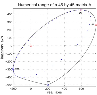
Normalization then gives two unit vector generators as desired. A set of great circle image points (•) and their two real axis crossings (+) are depicted in Figure 1 for a
specific matrixAthat will be described in the next section.
If, unlike Figure 1, none of the feasible ellipses gives us two real axis numerical range points to either side of zero initially, then we check whether their collective set does. If not, we compute more eigenanalyses forA(θ) = cos(θ)H(A) + sin(θ) iK(A) with angles θ other than θ = 0 and θ = π/2 as done at start-up with H(A) and iK(A), respectively. If for example all original ellipses intersect the real axis to the right of zero and ℑ(rm) <0, then we bisect the third quadrant and compute the largest eigenvalue and associated eigenvectorxnew ofA(3π/4) to find a∂F(A) point
that lies between iM and rm. If this point lies below the real axis, then we check the ellipse intersections of the great circle images through the generating vector of iM and xnew, otherwise we do the same for the generator of rm and xnew. Thus,
−200 0 200 400 600 −500
−400 −300 −200 −100 0 100 200 300 400
Numerical range of a 45 by 45 matrix A
real axis
imaginary axis
iM
im
rM
rm
Figure 2.1.Numerical range boundary(–)with extreme horizontal extension∂F(A)pointsrm ()andrM (), and extreme vertical extensions ofF(A)atiM()andim(). Image points(•) of the great circle through the generating vectors ofiMandrm, and its real axis crossings(+)(and an earlier one). Zero inCato.
angle bisection has generally been low, normally below 4 and possibly up into the teens only when zero lies within 10−13of the boundary∂F(A) in absolute terms.
Overall, the most expensive parts of our algorithm are the eigenanalyses ofA(θ) at O(n3) cost. The remainder of the program requires a number of quadratic form
evaluations in the form of x∗
A y as in Proposition 1.1(a) and in equations (2.1) and (2.2) atO(n2) cost, as well as sorts, finds etc at even lowerO(n) orO(1) computational
cost.
3. Tests. The 45×45 complex matrix whose numerical range is depicted in Figure 2.1 is constructed from the complex matrix B ∈C45×45 in [9, p. 463]. This
matrix B is the sum of the Fiedler matrix F = (|i−j|) and i times the Moler matrix M = UTU for the upper triangular matrix U with u
i,j = −1 for j >
the algorithms of [2, 13] and our algorithm:
n= 45 execution time eigenanalyses error |x∗A x−0|
wberpointfrom [13] 0.1 to 0.15 sec 3 10−10 to 9·10−11
inversefovfrom [2] 0.0071 sec 3 3.6·10−13
this paper’s algorithm 0.0042 sec 2 2.3·10−13
Table 1
Note thatwberpointrelies on randomly generated vectors inCnand therefore its run
data will vary with the chosen random vectors accordingly. For the same type of 500× 500 matrixB, we consider the matrix generated by A=B+(-3+5i)*ones(500)-(-200 +500i)*eye(500)and denote it byA500,500. The computed data is as follows:
n= 500 execution time eigenanalyses error |x∗A x−0|
wberpointfrom [13] 2.3 to 4.8 sec 0 to 1 (eigs) 5·10−10 to 4·10−12 inversefovfrom [2] 0.75 sec 2 (eig) 3.7·10−11
this paper’s algorithm 0.24 sec 4 (eigs) 6·10−13
Table 2
The 500×500 matrixA500,500has one tight cluster of 493 relatively small eigenvalues
of magnitudes around 540 and 7 separate eigenvalues of increasing magnitudes up to 11.2·104. Our inverse numerical range routine as well as those of [2, 13] use
the Krylov type eigensolvereigsin MATLAB for large dimensional matrices A for its better speed in finding the largest and/or smallest eigenvalue(s) ofA(θ) that we need. Since all iteration matrices A(θ) = cos(θ)H(A) + sin(θ) iK(A) are hermitian, their eigenvalues are well conditioned. But their tight clustering and large magnitude discrepancies make the Lanczos method ofeigsquite unsuitable when used with the MATLAB default setting for the Ritz estimate residual tolerance opts.tol to the machine constant eps= 2.2. ·10−16. To gain convergence ofeigs in our algorithm
for A500,500 we have to use opts.tol values between 10−5 and 10−3 instead. This
apparently has no ill effect on our inverse problem accuracy. Likewise changing the opts.tolsetting inside the code of [2] does, however, not help since its call ofeigs crashes. Therefore, the current codeinversefovin [2] is of limited use in clustered eigen-situations. On the other hand, [2] works well as does ours, when using the much more expensive Francis QR based dense eigensolvereigof MATLAB. Note that our code with its very loose Lanzcos based eigensolver still obtains a generating vector for µ that is almost two orders of magnitude better than what eigcan achieve in inversefovfrom [2]. Finally, if we use our code with eiginstead for thisA500,500,
the run time will go up comparably but the error comes in at only around 3.5·10−12.
−25 −20 −15 −10 −5 0 5 −20
−15 −10 −5 0 5 10
Numerical range of a 10 by 10 matrix A
real axis
imaginary axis
rM iM
rm
im
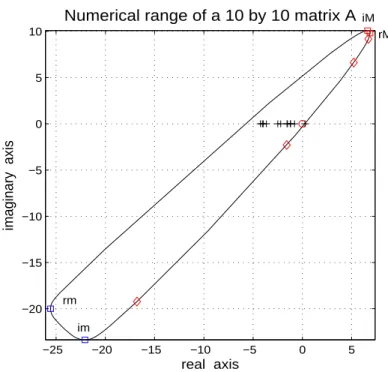
Figure 3.1. Numerical range boundary(–) with extreme horizontal extension ∂F(A−µ I10) points rm () and rM (), and extreme vertical extensions at iM () and im(). Numerical range real axis points(+): several to the left and one to the right of zero, as well as intermediate
∂F(A)points(♦)of4angle bisecting steps.
in Figure 3.1, where we have shifted the origin by µ= 22.5 + i 20.
For the chosen µ= 22.5 + i 20, our method finds a generating vector after 4 angle bisections since according to Figure 3.1 then there are known generating vectors for real axis points to the left and right of zero and Proposition 1.1 applies. If we move µcloser to the edge ofF(A) by increasingℜ(µ), the computed data for this example is as follows:
µ C number inversefovfrom [2] this paper’s algorithm sec eig error sec eig error 22.83543 + i 20 −5·10−8 0.09 12 8·10−13 0.045 14 10−15 22.835430065 + i 20 −3·10−
10
0.11 17 5·10−
12
0.045 14 3.6·10−
15
22.8354300651 + i 20 −2.4·10−
10
0.21 35 3·10−
12
0.047 14 10−15
22.835430065417 + i 20 −7·10−13 * * * 0.049 16 10−15 22.835430065418 + i 20 4·10−
13
* * * µ outside F(A)
Here the ‘C number’ denotes the generalized Crawford number and indicates the minimal distance ofµfrom the boundary of the numerical range of A−µ I10. It was
computed viaCraw2circ.mof [15, 16]. As long as the generalized Crawford number of a given point µ∈C is negative, the point lies inside the numerical range. The third
data row of the Table 3 exhibits the best that could be achieved withinversefovfrom [2]; ifµis changed to 22.8354300652 + i 20 for example, inversefovfails altogether while our algorithm works correctly for three more digits or 15 digit precision in µ. Note how the origin approaches∂F(A) in successive data rows from order 10−8 to
order 10−13, and that in our algorithm the number of eigenanalyses hardly increases
here. The 5th data line above indicates that our algorithm determined that the point µ= 22.835430065418 + i20 to lie outside the numerical range ofAwith a distance of order 4·10−13 from its boundary. This also took 16 eigenanalyses.
Our last example comes from [13, Example 7] and uses a 188×188 Jordan block J for the eigenvalue 1 + i 3 (with all co-diagonals equal to 1) as test matrix. Here, both [2] and our algorithm use 3 eigenanalyses; our algorithm finds a generating unit vector for the point µ= 1.707 + i 3.707 that lies insideF(A) within 10−5of∂F(A) in
0.17 seconds with accuracy of order 10−17while
inversefovfrom [2] uses 0.2 seconds with 9·10−16 accuracy. For this example, wberpointof [13, Example 7] achieves an
accuracy of 3.8·10−10 in almost 1 second and uses 7 eigenanalyses.
4. Conclusions and comments. We have developed, implemented and tested a short, quick and accurate inverse numerical range algorithm that finds a generating complex unit vector of any field of values point in its interior. The proposed method relies on geometric ideas for computations in the realm of the matrix numerical range and is frugal with itsO(n3) eigenanalyses that are – at this time – apparently necessary
to proceed here.
To also look for imaginary axis field of values points below and above µ in the complex plane and their generators might offer another, quite natural improvement as well, but first tries with a thus expanded version of our subroutineCvectinterpol inside [14] have shown but little speed-up, if any, and that idea has been abandoned.
Finally, we remark that our code was tested using MATLAB2009b on both MACs and PCs.
REFERENCES
[1] C.A. Beattie, M. Embree, and D.C. Sorensen. Convergence of polynomial restart Krylov methods for eigenvalue computations. SIAM Rev., 47:492–515, 2003.
[3] C. Davis. The Toeplitz-Hausdorff Theorem explained.Canad. Math. Bull., 14:245–246, 1971.
[4] M. Eiermann. Field of values and iterative methods.Linear Algebra Appl., 180:167–197, 1993.
[5] M. Embree and L.N. Trefethen.Spectra and Pseudospectra: The Behavior of Nonnormal Matrices and Operators. Princeton University Press, 2005.
[6] M. Goldberg and E. Tadmor. On the numerical radius and its applications. Linear Algebra Appl., 42:263–284, 1982.
[7] K.E. Gustafson and D.K.M. Rao. Numerical Range, The Field of Values of Linear Operators and Matrices. Springer-Verlag, New York, 1997.
[8] F. Hausdorff. Der Wertvorrat einer Bilinearform. Math. Z., 3:314–316, 1919.
[9] N.J. Higham, F. Tisseur, and P.M. van Dooren. Detecting a definite hermitian pair and a hyperbolic or elliptic quadratic eigenvalue problem, and associated nearness problems. Linear Algebra Appl., 351/352:455–474, 2002.
[10] R.A. Horn and C.R. Johnson.Topics in Matrix Analysis. Cambridge University Press, Cambridge, 1991.
[11] C.R. Johnson. Numerical determination of the field of values of a general complex matrix. Linear Algebra Appl., 15:595–602, 1978.
[12] O. Toeplitz. Das algebraische Analogon zu einern Satze von Fej´er.Math. Z., 2:187–197, 1918.
[13] F. Uhlig. An inverse field of values problem. Inverse Problems, 25:055019, 2008. [14] F. Uhlig. MATLAB m-fileinvfovCPU.m, 2010. Available at http://www.auburn.edu/
˜uhligfd/m files/invfovCPU.m.
[15] F. Uhlig. On computing the generalized Crawford number of a matrix. Submitted. [16] F. Uhlig. MATLAB m-fileCraw2circ.m, 2010. Available at http://www.auburn.edu/