ISSN1842-6298 (electronic), 1843 - 7265 (print) Volume3(2008), 111 – 122
THE EFFICIENCY OF MODIFIED JACKKNIFE
AND RIDGE TYPE REGRESSION ESTIMATORS: A
COMPARISON
Feras Sh. M. Batah, Thekke V. Ramanathan and Sharad D. Gore
Abstract. A common problem in multiple regression models is multicollinearity, which pro-duces undesirable effects on the least squares estimator. To circumvent this problem, two well known estimation procedures are often suggested in the literature. They are Generalized Ridge Regression (GRR) estimation suggested by Hoerl and Kennard [8] and the Jackknifed Ridge Regression (JRR) estimation suggested by Singh et al. [13]. The GRR estimation leads to a reduction in the sampling variance, whereas, JRR leads to a reduction in the bias. In this paper, we propose a new estimator namely, Modified Jackknife Ridge Regression Estimator (MJR). It is based on the criterion that combines the ideas underlying both the GRR and JRR estimators. We have investigated standard properties of this new estimator. From a simulation study, we find that the new estimator often outperforms the LASSO, and it is superior to both GRR and JRR estimators, using the mean squared error criterion. The conditions under which the MJR estimator is better than the other two competing estimators have been investigated.
1
Introduction
One of the major consequences of multicollinearity on the ordinary least squares (OLS) method of estimation is that it produces large variances for the estimated re-gression coefficients. For improving the precision of the OLS estimator, two standard procedures are (i) the Generalized Ridge Regression (GRR) and (ii) the Jackknifed Ridge Regression (JRR). The method of ridge regression is one of the most widely used ”ad hoc” solution to the problem of multicollinearity (Hoerl and Kennard, [8]). The principle result concerning the ridge estimator is that, it is superior to the OLS estimator in terms of sampling variance even though biased. Hoerl and Kennard [8] and later Vinod [15] examined the performance of the ridge estimator using the MSE
2000 Mathematics Subject Classification:62J05; 62J07.
Keywords: Generalized Ridge Regression; Jackknifed Ridge Regression; Mean Squared Error; Modified Jackknife Ridge Regression; Multicollinearity
criterion and showed that there always exists a ridge estimator having smaller MSE than the OLS estimator (see also Vinod and Ullah [16] in this context). Hinkley [7] proposed a Jackknife method for multiple linear regression which later extended to Jackknifed ridge regression by Singh et al. [13]. Gruber [5] compared the Hoerl and Kennard ridge regression estimator with the Jackknifed ridge regression estimator and observed that, although the use of the Jackknife procedure reduces the bias considerably, the estimators may have large variances and MSE than the ordinary ridge regression estimators in certain situations. More recently it has been shown that effect Batah et al. [2] and improving precision for Jackknifing ridge type es-timation Batah and Gore [1]. In this paper, we have suggested a new estimator for the regression parameter by modifying the GRR estimator in the line of JRR estimator. Some important properties of this estimator are studied. Further, we have established the MSE superiority of the proposed estimator over both the GRR and the JRR estimators. We have also derived conditions for MSE superiority of this estimator. The paper is organized as follows: The model as well as the GRR and the JRR estimators are described in Section 2. The proposed new estimator is introduced in Section3. The performance of this estimator vis-a-vis the GRR and the JRR estimators are studied in Section4. Section5considers a small simulation study to justify the superiority of the suggested estimator. The paper ends with some conclusions in Section6.
2
The Model, GRR and JRR Estimators
Consider a multiple linear regression model
Y =Xβ+ǫ, (2.1)
where Y is an (n×1) vector of observations on the dependent variable, X is an (n×p) matrix of observations on p non-stochastic independent variables, β is a (p×1) vector of parameters associated with the p regressors and ǫ is an (n×1) vector of disturbances having mean zero and variance-covariance matrixσ2In. We assume that two or more regressors in X are closely linearly related, so that the model suffers from the problem of multicollinearity. Let Λ and T be the matrices of eigenvalues and eigenvectors of X′X, then T′X′XT = Λ =diag(λ
1, λ2, . . . , λp), λi being the i-th eigenvalue ofX′X and T′T =T T′ =I. The orthogonal version of the model (2.1) is
Y =Zγ+ǫ, (2.2)
where Z = XT and γ = T′β, using singular value decomposition (see, Vinod and Ullah, [16, p. 5] of X. The OLS estimator ofγ is given by
ˆ
γ(LS)= (Z′Z)−1Z′Y
Since γ=T′β and T′T =I,the OLS estimator of β is given by
By jackknifing the GRR estimator (2.5), Singh et al. [13] proposed the JRR esti-mator:
ˆ
γJ(K) = (I+KA−1)ˆγR(K) = (I−K2A−2)ˆγ(LS). (2.8)
When k1 = k2 = . . . = kp = k, k > 0 the ordinary Jackknifed ridge regression (OJR) estimator of γ can be written as
Obviously, the OLS estimator refers to the case whereki= 0. It is easily seen from
In this section, a new estimator of γ is proposed. The proposed estimator is des-ignated as the Modified Jackknife Ridge Regression estimator (MJR) denoted by ˆ
γM J(K):
ˆ
γM J(K) = [I−K2A−2]ˆγR(K) = [I−K2A−2][I−KA−1]ˆγ(LS). (3.1)
When k1 = k2 = . . . = kp = k, k > 0 the MJR estimator is called the Modified Ordinary Jackknife Ridge Regression estimator (MOJR) denoted by ˆγM J(k):
ˆ
γM J(k) = [I −k2Ak−2][I−kA−1k ]ˆγ(LS).
Obviously, ˆγiM J(K) = ˆγ(iLS) when ki = 0. It may be noted that the proposed estimator MJR in (3.1) is obtained as in the case of JRR estimator - but with GRR instead of OLS. Accordingly, from (2.10)
The MJR estimator is also the Bayes estimator, if each γi independently follow a normal prior with E(γi) = 0 andV ar(γi) = f(k
i)
1−f(ki)
σ2
λi with f(ki) as given in (3.2).
The expressions for bias, variance and mean squared errors may be obtained as below:
Bias
Bias(ˆγM J(K)) =E(ˆγM J(K))−γ =−K[I+KA−1−KA−2K]A−1γ. (3.3)
Variance
V ar(ˆγM J(K)) = E[(ˆγM J(K)−E(ˆγM J(K)))(ˆγM J(K)−E(ˆγM J(K)))′]
= σ2WΛ−1W′, (3.4)
whereW = (I−K2A−2)(I−KA−1).
Mean Squared Error (MSE)
M SE(ˆγM J(K)) = V ar(ˆγM J(K)) + [Bias(ˆγM J(K))][Bias(ˆγM J(K))]′ = σ2WΛ−1W′+KΦA−1γγ′A−1Φ′K. (3.5)
where Φ = [I+KA−1−KA−2K].
4
The Performance of the MJR Estimator by MSE
Cri-terion
We have already seen in the previous section that, the estimator MJR is biased and hence the appropriate criterion for gauging the performance of this estimator is MSE. Next, we compare the performance of the MJR estimator vis-a-vis the GRR and the JRR estimators by this criterion.
4.1 Comparison between the MJR and the GRR estimators
As regards the performance by the sampling variance, we have the following theorem.
Theorem 1. Let K be a (p×p) symmetric positive definite matrix. Then the MJR estimator has smaller variance than the GRR estimator.
Proof. From (2.14) and (3.4) it can be shown that
where
H = (I −KA−1)Λ−1(I−KA−1)′[I−(I−K2A−2)(I−K2A−2)]
= (I −KA−1)Λ−1(I−KA−1)′[(I−(I −K2A−2))(I+ (I−K2A−2))] = (I −KA−1)Λ−1(I−KA−1)′[K2A−2(I+ (I−K2A−2))] (4.1)
and A = Λ +K. Since A−1 is positive definite, (I −KA−1) and (I −K2A−2) are positive definite matrices. It can be concluded that the matrix [I + (I −K2A−2)] is positive definite so that multiplying by [K2A−2[I+ (I−K2A−2)]] will result in a positive definite matrix. Thus, we conclude thatH is positive definite wheneverK (p×p) is a symmetric positive definite matrix. This completes the proof.
Next we prove a necessary and sufficient condition for the MJR estimator to outper-form the GRR estimator using the MSE criterion. The proof requires the following lemma from Groß[4, p.356].
Lemma 2. LetAbe a symmetric positive definitep×pmatrix,γ anp×1vector and
αa positive number. ThenαA−γγ′is nonnegative definite if and only ifγ′A−1γ ≤α
is satisfied.
Theorem 3. Let K be a (p×p) symmetric positive definite matrix. Then the difference
∆ =M SE(γ,γRˆ (K))−M SE(γ,γM Jˆ (K))
is a nonnegative definite matrix if and only if the inequality
γ′[L−1(σ2H+KA−1γγ′A−1K)L−1]−1γ ≤1, (4.2)
is satisfied with L = K(I +KA−1−KA−2K)A−1. In addition, ∆ 6= 0 whenever
p >1.
Proof. From (2.17) and (3.5) we have
∆ = M SE(γ,γˆR(K))−M SE(γ,γˆM J(K))
= σ2H+KA−1γγ′A−1K−KΦA−1γγ′A−1Φ′K, (4.3)
where Φ = (I+KA−1−KA−2K) is a positive definite matrix. We have seen thatHis positive definite from Theorem1. Therefore, the difference ∆ =M SE(γ,γˆR(K))− M SE(γ,γM Jˆ (K)) is a nonnegative definite if and only if L−1∆L−1 is nonnegative definite. The matrixL−1∆L−1 can be written as
Since the matrix (σ2H + KA−1γγ′A−1K) is symmetric positive definite, using Lemma 2, we may conclude that L−1∆L−1 is nonnegative definite if and only if the inequality
γ′[L−1(σ2H+KA−1γγ′A−1K)L−1]−1γ ≤1, (4.5)
is satisfied. Moreover, ∆ = 0 if and only ifL−1∆L−1= 0, that is
L−1(σ2H+KA−1γγ′A−1K)L−1 =γγ′. (4.6)
The rank of the left hand matrix is p, while the rank of the right hand matrix is either 0 or 1. Therefore ∆ = 0 cannot hold true whenever p >1. This completes the proof.
For the special caseK =kIp, the inequality
γ′[L−1(σ2H+KA−1γγ′A−1K)L−1]−1γ≤1,
becomes
γ′[L−1 k (σ
2H
k+k2A−k1γγ′Ak−1)L−k1]−1γ ≤1,
is satisfied, where
Lk =k(I+kA−1k −k2A−2k )A−1k ,
and
H= (I−kA−1k )Λ−1(I−kA−1 k )′[k
2A−2
k (I + (I−k 2A−2
k ))].
In addition, ∆6= 0 wheneverk >0 and p >1.
4.2 Comparison between the MJR and the JRR estimators
Here we show that the MJR estimator outperform the JRR estimator in terms of the sampling variance.
Theorem 4. Let K be a (p×p) symmetric positive definite matrix. Then the MJR estimator has smaller variance than the JRR estimator.
Proof. From (2.16) and (3.4) it can be shown that V ar(ˆγJ(K))−V ar(ˆγM J(K)) =
σ2Ω, where
Ω = (I −K2A−2)Λ−1(I−K2A−2)′[KA−1(I+ (I−KA−1))]. (4.7)
Rewriting the arguments leads to the conclusion that Ω is positive definite whenever K is a (p×p) symmetric positive definite matrix and hence the proof.
Theorem 5. Let K be a (p×p) symmetric positive definite matrix. Then the difference
∆ =M SE(γ,γˆJ(K))−M SE(γ,γˆM J(K))
is a nonnegative definite matrix if and only if the inequality
γ′[L−1(σ2Ω +K2A−2γγ′A−2K2)L−1]−1γ ≤1, (4.8)
is satisfied. In addition, ∆6= 0 whenever p >1.
Remark 6. It may be noted that (4.2) and (4.8) are complex functions of K, as
well as they depend on unknown parameters β and σ2. And hence, it is difficult to
establish the existence of K from (4.2) and (4.8). However, it may be guaranteed
that when K = kIp, with k > 0, these conditions are trivially met. (Infact, it can
be shown that when k→0, the condition fails and otherwise it holds good, including
when k→ ∞).
5
A Simulation Study
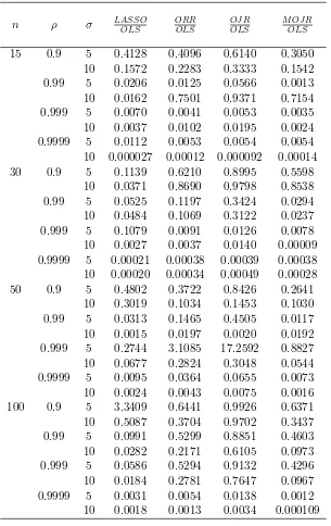
In this section, we present a Monte Carlo study to compare the mean of the rela-tive mean squared error of four estimators viz., LASSO (Least Absolute Shrinkage and Selection Operator) suggested in Tibshirani [14], ORR, OJR and MOJR with OLS. All simulations were conducted using MATLAB code. Eachβj is rewritten as βi+−β−
i , whereβi+ andβ−i are nonnegative. We have used the quadratic program-ming module ’quadprog’ in MATLAB to find the LASSO solution. The true model Y = Xβ+σǫ, is considered with β = (1,0,1)′. Here ǫ follows a standard normal distributionN(0,1) and the explanatory variables are generated from
xij = (1−ρ2)
1
2wij +ρwip, i= 1,2, . . . , n; j = 1,2, . . . , p, (5.1)
where wij are independent standard normal random numbers and ρ2 is the corre-lation between xij and xij′ for j, j′ < p and j 6= j′, j, j′ = 1,2, . . . , p. When j or
Our simulation is patterned as in McDonald and Galarneau [11] and Leng et al. [10]. This pattern was also adopted by Wichern and Churchill [17], and Gibbons [3]. When computing the estimator, we first transform the original linear model to canonical form to get the estimator ofγ. Then the estimator ofγis transformed back to the estimator ofβ. For each choice of ρ, σ2 and n, the experiment is replicated 1000 times and obtained the average MSE:
M SE( ˆβi) = 1 1000
1000X
j=1
( ˆβij −βi)2, (5.2)
where ˆβij denote the estimate of the i-th parameter in j-th replication and β1, β2 and β3 are the true parameter values. Numerical results of the simulation are sum-marized in Table1. It may be noted that the performance of MOJR is excellent in comparison with that of the other estimators for all combinations of correlation be-tween regressors and variance of errorsσ2,except with LASSO estimator (cf. Table
1). With LASSO, the suggested MOJR estimator has a mixed performance pattern in terms of MSE.
Remark 7. Extensive simulations were carried out to study the behavior of the MOJR in comparison with the other estimators when the correlations are low with
smallerσ. We have observed that the performance of MOJR estimator is quite good
in those cases. When σ is large, the MSE of MOJR estimator is still comparable
with the other two estimators, even if they are on the higher side.
Remark 8. It may be noted that the R2 value of the analysis is quite sensitive to
the choice of σ2. This observation was also made by Peele and Ryan [12]. In our
simulation study, we have observed that the R2 values were between 0.55 - 0.90 for
all choices of σ2.
Remark 9. Even though the MOJR estimator does not always perform better than the LASSO estimator, their MSE’s are comparable. However, it may be noted that, it is possible to derive an exact analytical expression for the MSE of MOJR estimator, whereas, in the case of LASSO, it is simply not possible.
6
Conclusion
n ρ σ LASSOOLS ORROLS OJ ROLS M OJ ROLS
15 0.9 5 0.4128 0.4096 0.6140 0.3050 10 0.1572 0.2283 0.3333 0.1542 0.99 5 0.0206 0.0125 0.0566 0.0013 10 0.0162 0.7501 0.9371 0.7154 0.999 5 0.0070 0.0041 0.0053 0.0035 10 0.0037 0.0102 0.0195 0.0024 0.9999 5 0.0112 0.0053 0.0054 0.0054 10 0.000027 0.00012 0.000092 0.00014 30 0.9 5 0.1139 0.6210 0.8995 0.5598
10 0.0371 0.8690 0.9798 0.8538 0.99 5 0.0525 0.1197 0.3424 0.0294 10 0.0484 0.1069 0.3122 0.0237 0.999 5 0.1079 0.0091 0.0126 0.0078 10 0.0027 0.0037 0.0140 0.00009 0.9999 5 0.00021 0.00038 0.00039 0.00038 10 0.00020 0.00034 0.00049 0.00028 50 0.9 5 0.4802 0.3722 0.8426 0.2641
10 0.3019 0.1034 0.1453 0.1030 0.99 5 0.0313 0.1465 0.4505 0.0117 10 0.0015 0.0197 0.0020 0.0192 0.999 5 0.2744 3.1085 17.2592 0.8827 10 0.0677 0.2824 0.3048 0.0544 0.9999 5 0.0095 0.0364 0.0655 0.0073 10 0.0024 0.0043 0.0075 0.0016 100 0.9 5 3.3409 0.6441 0.9926 0.6371 10 0.5087 0.3704 0.9702 0.3437 0.99 5 0.0991 0.5299 0.8851 0.4603 10 0.0282 0.2171 0.6105 0.0973 0.999 5 0.0586 0.5294 0.9132 0.4296 10 0.0184 0.2781 0.7647 0.0967 0.9999 5 0.0031 0.0054 0.0138 0.0012 10 0.0018 0.0013 0.0034 0.000109
Table 1:
Ratio of MSE of estimators when ˆk= pˆσ
2 (J)
ˆ
the superiority of this estimator over the other two estimators in terms of MSE. We have established that this suggested estimator has a smaller mean square error value than the GRR and JRR estimators. Even though the MJR estimator does not always perform better than LASSO estimator, their MSE’s are comparable.
Acknowledgement. The first author wishes to thank the Indian Council for Cultural Relations (ICCR) for the financial support. The authors would like to acknowledge the editor and the referee for their valuable comments, which improved the paper substantially.
References
[1] F. Batah and S. Gore, Improving Precision for Jackknifed Ridge Type Estima-tion, Far East Journal of Theoretical Statistics 24(2008), No.2, 157–174.
[2] F. Batah, S. Gore and M. Verma,Effect of Jackknifing on Various Ridge Type
Estimators, Model Assisted Statistics and Applications3 (2008), To appear.
[3] D. G. Gibbons,A Simulation Study of Some Ridge Estimators, Journal of the American Statistical Association76 (1981), 131 – 139.
[4] J. Groß, Linear Regression: Lecture Notes in Statistics, Springer Verlag, Ger-many, 2003.
[5] M. H. J. Gruber,The Efficiency of Jackknife and Usual Ridge Type Estimators:
A Comparison, Statistics and Probability Letters11 (1991), 49 – 51.
[6] M. H. J. Gruber, Improving Efficiency by Shrinkage: The James-Stein and
Ridge Regression Estimators, New York: Marcel Dekker, Inc, 1998.MR1608582
(99c:62196) . Zbl 0920.62085.
[7] D. V. Hinkley,Jackknifing in Unbalanced Situations, Technometrics19(1977), No. 3, 285 – 292. Zbl 0367.62085 .
[8] A. E. Hoerl and R. W. Kennard,Ridge Regression: Biased Estimation for Non
orthogonal Problems, Technometrics 12(1970), 55 – 67.Zbl 0202.17205.
[9] A. Hoerl, R. Kennard and K. Baldwin, Ridge Regression: Some Simulations, Commun. Statist. Theor. Meth. 4 (1975), 105–123.
[10] C. Leng, Yi Lin and G. Wahba , A Note on the Lasso and Related Procedures
in Model Selection, Statistica Sinica 16 (2006), 1273–1284. MR2327490. Zbl
1109.62056.
[11] G. C. McDonald and D. I. Galarneau,A Monte Carlo Evaluation of Some
Ridge-type Estimators, Journal of the American Statistical Association 70 (1975),
[12] L. C. Peele and T. P. Ryan ,Comments to: A Critique of Some Ridge Regression
Methods, Journal of the American Statistical Association75(1980), 96–97.Zbl
0468.62065.
[13] B. Singh, Y. P. Chaube and T. D. Dwivedi, An Almost Unbiased Ridge
Esti-mator, Sankhya Ser.B 48(1986), 342–346. MR0905210(88i:62124).
[14] R. Tibshirani,Regression Shrinkage and Selection via the Lasso, Journal of the Royal Statistical Society B, 58 (1996), 267–288. MR1379242 (96j:62134). Zbl 0850.62538.
[15] H. D. Vinod, A Survey for Ridge Regression and Related Techniques for
Im-provements Over Ordinary Least Squares, The Review of Economics and
Statis-tics 60(1978), 121–131. MR0523503(80b:62085).
[16] H. D. Vinod and A. Ullah,Recent Advances in Regression Methods, New York: Marcel Dekker Inc, 1981. MR0666872 (84m: 62097).
[17] D. Wichern and G. Churchill,A Comparison of Ridge Estimators, Technomet-rics 20(1978), 301–311. Zbl 0406.62050.
Feras Shaker Mahmood Batah Thekke Variyam Ramanathan Department of Statistics, University of Pune, India. Department of Statistics, Department of Mathematics, University of Alanber, Iraq. University of Pune, India.
e-mail: [email protected] e-mail: [email protected]
Sharad Damodar Gore