El e c t ro n ic
Jo ur n
a l o
f P
r o b
a b i l i t y
Vol. 12 (2007), Paper no. 25, pages 703–766. Journal URL
http://www.math.washington.edu/~ejpecp/
Distances in random graphs with finite mean and
infinite variance degrees
Remco van der Hofstad∗†
Gerard Hooghiemstra‡ and Dmitri Znamenski§†
Abstract
In this paper we study typical distances in random graphs with i.i.d. degrees of which the tail of the common distribution function is regularly varying with exponent 1−τ. Depending on the value of the parameterτ we can distinct three cases: (i) τ >3, where the degrees have finite variance, (ii)τ∈(2,3), where the degrees have infinite variance, but finite mean, and (iii)τ ∈(1,2), where the degrees have infinite mean. The distances between two randomly chosen nodes belonging to the same connected component, for τ >3 and τ ∈(1,2), have been studied in previous publications, and we survey these results here. Whenτ ∈(2,3), the graph distance centers around 2 log logN/|log(τ−2)|. We present a full proof of this result, and study the fluctuations around this asymptotic means, by describing the asymptotic distribution. The results presented here improve upon results of Reittu and Norros, who prove an upper bound only.
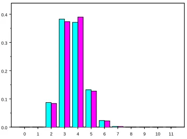
The random graphs studied here can serve as models for complex networks where degree power laws are observed; this is illustrated by comparing the typical distance in this model to Internet data, where a degree power law with exponentτ ≈ 2.2 is observed for the so-called Autonomous Systems (AS) graph .
Key words: Branching processes, configuration model, coupling, graph distance.
∗Department of Mathematics and Computer Science, Eindhoven University of Technology, P.O. Box 513, 5600
MB Eindhoven, The Netherlands. E-mail: [email protected]
†Supported in part by Netherlands Organization for Scientific Research (NWO).
‡Delft University of Technology, Electrical Engineering, Mathematics and Computer Science, P.O. Box 5031,
2600 GA Delft, The Netherlands. E-mail: [email protected]
1
Introduction
Complex networks are encountered in a wide variety of disciplines. A rough classification has been given by Newman (18) and consists of: (i) Technological networks, e.g. electrical power grids and the Internet, (ii) Information networks, such as the World Wide Web, (iii) Social networks, like collaboration networks and (iv) Biological networks like neural networks and protein interaction networks.
What many of the above examples have in common is that the typical distance between two nodes in these networks are small, a phenomenon that is dubbed the‘small-world’phenomenon. A second key phenomenon shared by many of those networks is their‘scale-free’nature; meaning that these networks have so-called power-law degree sequences, i.e., the number of nodes with degree k falls of as an inverse power of k. We refer to (1; 18; 25) and the references therein for a further introduction to complex networks and many more examples where the above two properties hold.
A random graph model where both the above key features are present is the configuration model applied to an i.i.d. sequence of degrees with a power-law degree distribution. In this model we start by sampling the degree sequence from a power law and subsequently connect nodes with the sampled degree purely at random. This model automatically satisfies the power law degree sequence and it is therefore of interest to rigorously derive the typical distances that occur. Together with two previous papers (10; 14), the current paper describes the random fluctuations of the graph distance between two arbitrary nodes in the configuration model, where the i.i.d. degrees follow a power law of the form
P(D > k) =k−τ+1L(k),
where L denotes a slowly varying function and the exponent τ satisfies τ ≥ 1. To obtain a complete picture we include a discussion and a heuristic proof of the results in (10) forτ ∈[1,2), and those in (14) forτ > 3. However, the main goal of this paper is the complete description, including a full proof of the case where τ ∈ (2,3). Apart from the critical cases τ = 2 and τ = 3, which depend on the behavior of the slowly varying function L (see (10, Section 4.2) when τ = 2), we have thus given a complete analysis for all possible values of τ ≥1.
This section is organized as follows. In Section 1.1, we start by introducing the model, in Section 1.2 we state our main results. Section 1.3 is devoted to related work, and in Section 1.4, we describe some simulations for a better understanding of our main results. Finally, Section 1.5 describes the organization of the paper.
1.1 Model definition
Fix an integerN. Consider an i.i.d. sequence D1, D2, . . . , DN. We will construct an undirected
graph withN nodes where nodej has degreeDj. We assume thatLN =
PN
j=1Dj is even. IfLN
is odd, then we increase DN by 1. This single change will make hardly any difference in what
follows, and we will ignore this effect. We will later specify the distribution ofD1.
To construct the graph, we have N separate nodes and incident to node j, we have Dj stubs
LN −1 remaining stubs. Once paired, two stubs (half-edges) form a single edge of the graph.
Hence, a stub can be seen as the left or the right half of an edge. We continue the procedure of randomly choosing and pairing the stubs until all stubs are connected. Unfortunately, nodes having self-loops may occur. However, self-loops are scarce whenN → ∞, as shown in (5). The above model is a variant of the configuration model, which, given a degree sequence, is the random graph with that given degree sequence. The degree sequence of a graph is the vector of which thekth coordinate equals the proportion of nodes with degree k. In our model, by the
law of large numbers, the degree sequence is close to the probability mass function of the nodal degree Dof which D1, . . . , DN are independent copies.
The probability mass function and the distribution function of the nodal degree law are denoted by
P(D1 =j) =fj, j= 1,2, . . . , and F(x) =
⌊x⌋
X
j=1
fj, (1.1)
where⌊x⌋is the largest integer smaller than or equal tox. We consider distributions of the form
1−F(x) =x−τ+1L(x), (1.2)
whereτ >1 andLis slowly varying at infinity. This means that the random variables Dj obey
a power law, and the factorL is meant to generalize the model. We assume the following more specific conditions, splitting between the casesτ ∈(1,2), τ ∈(2,3) andτ >3.
Assumption 1.1. (i) Forτ ∈(1,2), we assume (1.2).
(ii) Forτ ∈(2,3), we assume that there exists γ ∈[0,1) andC >0 such that
x−τ+1−C(logx)γ−1 ≤1−F(x)≤x−τ+1+C(logx)γ−1, for large x. (1.3)
(iii) Forτ >3, we assume that there exists a constant c >0 such that
1−F(x)≤cx−τ+1, for allx≥1, (1.4)
and that ν >1, where ν is given by
ν= E[D1(D1−1)]
E[D1]
. (1.5)
Distributions satisfying (1.4) include distributions which have a lighter tail than a power law, and (1.4) is only slightly stronger than assuming finite variance. The condition in (1.3) is slightly stronger than (1.2).
1.2 Main results
We define the graph distanceHN between the nodes 1 and 2 as the minimum number of edges
because the nodes are exchangeable. In order to state the main result concerningHN, we define
the centering constant
mτ,N=
(
2⌊|log loglog(τ−N2)|⌋, forτ ∈(2,3),
⌊logνN⌋, forτ >3. (1.6) The parameter mτ,N describes the asymptotic growth ofHN asN → ∞. A more precise result
including the random fluctuations aroundmτ,N is formulated in the following theorem.
Theorem 1.2 (The fluctuations of the graph distance). When Assumption 1.1 holds, then
(i) for τ ∈(1,2),
lim
N→∞P(HN = 2) = 1−Nlim→∞P(HN = 3) =p, (1.7)
where p=pF ∈(0,1).
(ii) for τ ∈(2,3) or τ >3 there exist random variables (Rτ,a)a∈(−1,0], such that as N → ∞,
PHN =mτ,N+l
HN <∞
=P(Rτ,aN =l) +o(1), (1.8)
where
aN =
(
⌊|log loglog(τ−N2)|⌋ −
log logN
|log(τ−2)|, for τ ∈(2,3), ⌊logνN⌋ −logνN, for τ >3.
We see that forτ ∈(1,2), the limit distribution exists and concentrates on the two points 2 and 3. Forτ ∈(2,3) orτ >3 the limit behavior is more involved. In these cases the limit distribution does not exist, caused by the fact that the correct centering constants, 2 log logN/(|log(τ−2)|), forτ ∈ (2,3) and logνN, forτ >3, are in general not integer, whereas HN is with probability
1 concentrated on the integers. The above theorem claims that for τ ∈ (2,3) or τ > 3 and largeN, we haveHN=mτ,N+Op(1), with mτ,N specified in (1.6) and whereOp(1) is a random
contribution, which is tight onR. The specific form of this random contribution is specified in Theorem 1.5 below.
In Theorem 1.2, we condition onHN <∞. In the course of the proof, here and in (14), we also
investigate the probability of this event, and prove that
P(HN<∞) =q2+o(1), (1.9)
whereq is the survival probability of an appropriate branching process.
Corollary 1.3 (Convergence in distribution along subsequences). For τ ∈(2,3) or τ >3, and when Assumption 1.1 is fulfilled, we have that, fork→ ∞,
HNk−mτ,Nk|HNk <∞ (1.10)
converges in distribution to Rτ,a, along subsequencesNk where aNk converges toa.
Corollary 1.4(Concentration of the hopcount). Forτ ∈(2,3) orτ >3, and when Assumption 1.1 is fulfilled, we have that the random variables HN−mτ,N, given that HN<∞, form a tight
sequence, i.e.,
lim
K→∞lim supN→∞ P
HN−mτ,N
≤K
HN <∞
= 1. (1.11)
We next describe the laws of the random variables (Rτ,a)a∈(−1,0]. For this, we need some further
notation from branching processes. Forτ >2, we introduce adelayedbranching process{Zk}k≥1,
where in the first generation the offspring distribution is chosen according to (1.1) and in the second and further generations the offspring is chosen in accordance tog given by
gj =
(j+ 1)fj+1
µ , j= 0,1, . . . , where µ=E[D1]. (1.12)
When τ ∈(2,3), the branching process {Zk} has infinite expectation. Under Assumption 1.1,
it is proved in (8) that
lim
n→∞(τ −2)
nlog(Z
n∨1) =Y, a.s., (1.13)
wherex∨y denotes the maximum ofx and y.
When τ >3, the process {Zn/µνn−1}n≥1 is a non-negative martingale and consequently
lim
n→∞
Zn
µνn−1 =W, a.s. (1.14)
The constantq appearing in (1.9) is the survival probability of the branching process{Zk}k≥1.
We can identify the limit laws of (Rτ,a)a∈(−1,0] in terms of the limit random variables in (1.13)
and (1.14) as follows:
Theorem 1.5 (The limit laws). When Assumption 1.1 holds, then
(i) for τ ∈(2,3) and for a∈(−1,0],
P(Rτ,a> l) =P
min
s∈Z
(τ−2)−sY(1)+(τ
−2)s−clY(2)
≤(τ−2)⌈l/2⌉+aY(1)Y(2)>0, (1.15)
where cl = 1 if l is even and zero otherwise, and Y(1), Y(2) are two independent copies of
the limit random variable in (1.13).
(ii) for τ >3 and for a∈(−1,0],
P(Rτ,a> l) =E
exp{−κν˜ a+lW(1)
W(2)
}W(1)
W(2) >0, (1.16)
where W(1) and
W(2) are two independent copies of the limit random variable
W in (1.14) and where ˜κ=µ(ν−1)−1.
The above results prove that the scaling in these random graphs is quite sensitive to the degree exponent τ. The scaling of the distance between pairs of nodes is proved for all τ ≥1, except for the critical cases τ = 2 and τ = 3. The result for τ ∈ (1,2), and the case τ = 1, where HN
P
τ ∈(2,3). Theorems 1.2-1.5 quantify the small-world phenomenon for the configuration model, and explicitly divide the scaling of the graph distances into three distinct regimes
In Remarks 4.2 and A.1.5 below, we will explain that our results also apply to the usual config-uration model, where the number of nodes with a given degree is deterministic, when we study the graph distance between two uniformly chosen nodes, and the degree distribution satisfied certain conditions. For the precise conditions, see Remark A.1.5 below.
1.3 Related work
There are many papers on scale-free graphs and we refer to reviews such as the ones by Albert and Barab´asi (1), Newman (18) and the recent book by Durrett (9) for an introduction; we refer to (2; 3; 17) for an introduction to classical random graphs.
Papers involving distances for the case where the degree distributionF (see (1.2)), has exponent τ ∈(2,3) are not so wide spread. In this discussion we will focus on the case whereτ ∈(2,3). For related work on distances for the casesτ ∈(1,2) andτ >3 we refer to (10, Section 1.4) and (14, Section 1.4), respectively.
The model investigated in this paper withτ ∈(2,3) was first studied in (21), where it was shown that with probability converging to 1, HN is less than mτ,N(1 +o(1)). We improve the results
in (21) by deriving the asymptotic distribution of the random fluctuations of the graph distance aroundmτ,N. Note that these results are in contrast to (19, Section II.F, below Equation (56)),
where it was suggested that if τ < 3, then an exponential cut-off is necessary to make the graph distance between an arbitrary pair of nodes well-defined. The problem of the mean graph distance between an arbitrary pair of nodes was also studied non-rigorously in (7), where also the behavior whenτ = 3 andx7→L(x) is the constant function, is included. In the latter case, the graph distance scales like log loglogNN. A related model to the one studied here can be found in (20), where a Poissonian graph process is defined by adding and removing edges. In (20), the authors prove similar results as in (21) for this related model. For τ ∈ (2,3), in (15), it was further shown that the diameter of the configuration model is bounded below by a constant times logN, whenf1+f2 >0, and bounded above by a constant times log logN, when f1+f2= 0.
A second related model can be found in (6), where edges between nodes i and j are present with probability equal towiwj/Plwl for some ‘expected degree vector’w= (w1, . . . , wN). It is
assumed that maxiw2i <
P
iwi, so that wiwj/Plwl are probabilities. In (6), wi is often taken
aswi=ci−
1
τ−1, wherecis a function ofN proportional toNτ−11 . In this case, the degrees obey a
power law with exponentτ. Chung and Lu (6) show that in this case, the graph distance between two uniformly chosen nodes is with probability converging to 1 proportional to logN(1 +o(1)) when τ > 3, and to 2|log loglog(τ−N2)|(1 +o(1)) when τ ∈ (2,3). The difference between this model and ours is that the nodes are not exchangeable in (6), but the observed phenomena are similar. This result can be heuristically understood as follows. Firstly, the actual degree vector in (6) should be close to the expected degree vector. Secondly, for the expected degree vector, we can compute that the number of nodes for which the degree is at leastk equals
|{i:wi≥k}|=|{i:ci−
1
τ−1 ≥k}| ∝k−τ+1.
0 1 2 3 4 5 6 7 8 9 10 11 0.0
0.1 0.2 0.3 0.4
Figure 1: Histograms of the AS-count and graph distance in the configuration model with N = 10,940, where the degrees have generating function fτ(s) in (1.18), for which the power
law exponentτ takes the valueτ = 2.25. The AS-data is lightly shaded, the simulation is darkly shaded.
assume some form of (conditional) independence of the edges, which results in asymptotic degree sequences that are given by mixed Poisson distributions (see e.g. (5)). In the configuration model, instead, thedegrees are independent.
1.4 Demonstration of Corollary 1.3
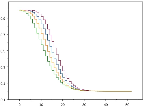
0 10 20 30 40 50 -0.1
0.1 0.3 0.5 0.7 0.9
Figure 2: Empirical survival functions of the graph distance forτ = 2.8 and for the four values of N.
Having motivated why we are interested to study distances in the configuration model, we now explain by a simulation the relevance of Theorem 1.2 and Corollary 1.3 forτ ∈(2,3). We have chosen to simulate the distribution (1.12) using the generating function:
gτ(s) = 1−(1−s)τ−2, for which gj = (−1)j−1
τ−2 j
∼ jτc−1, j→ ∞. (1.17)
Defining
fτ(s) =
τ−1 τ−2s−
1−(1−s)τ−1
τ−2 , τ ∈(2,3), (1.18) it is immediate that
gτ(s) =
fτ′(s) f′
τ(1)
, so that gj =
(j+ 1)fj+1
µ .
For fixed τ, we can pick different values of the size of the simulated graph, so that for each two simulated values N and M we have aN = aM, i.e., N = ⌈M(τ−2)
−k
⌉, for some integer k. For τ = 2.8, this induces, starting from M = 1000, by taking fork the successive values 1,2,3,
M = 1,000, N1 = 5,624, N2 = 48,697, N3= 723,395.
According to Corollary 1.3, the survival functions of the hopcountHN, given by k 7→ P(HN >
k|HN <∞), and forN =⌈M(τ−2)
−k
⌉, run approximately parallel on distance 2 in the limit for N → ∞, since mτ,Nk = mτ,M + 2k fork = 1,2,3. In Section 3.1 below we will show that the
1.5 Organization of the paper
The paper is organized as follows. In Section 2 we heuristically explain our results for the three different cases. The relevant literature on branching processes with infinite mean. is reviewed in Section 3, where we also describe the growth of shortest path graphs, and state coupling results needed to prove our main results, Theorems 1.2–1.5 in Section 4. In Section 5, we prove three technical lemmas used in Section 4. We finally prove the coupling results in the Appendix. In the sequel we will write that eventE occurswhpfor the statement thatP(E) = 1−o(1), as the total number of nodesN → ∞.
2
Heuristic explanations of Theorems 1.2 and 1.5
In this section, we present a heuristic explanation of Theorems 1.2 and 1.5.
When τ ∈(1,2), the total degree LN is the i.i.d. sum of N random variables D1, D2, . . . , DN,
with infinite mean. From extreme value theory, it is well known that then the bulk of the contribution toLN comes from a finitenumber of nodes which have giant degrees (the so-called
giant nodes). Since these giant nodes have degree roughly N1/(τ−1), which is much larger than
N, they are all connected to each other, thus forming a complete graph of giant nodes. Each stub of node 1 or node 2 is with probability close to 1 attached to a stub of some giant node, and therefore, the distance between any two nodes is, whp, at most 3. In fact, this distance equals 2 precisely when the two nodes are attached to thesamegiant node, and is 3 otherwise. Forτ = 1 the quotientMN/LN, where MN denotes the maximum of D1, D2, . . . , DN, converges
to 1 in probability, and consequently the asymptotic distance is 2 in this case, as basically all nodes are attached to the unique giant node. As mentioned before, full proofs of these results can be found in (10).
Forτ ∈(2,3) orτ >3 there are two basic ingredients underlying the graph distance results. The first one is that for two disjoint sets of stubs of sizesnandm out of a total ofL, the probability that none of the stubs in the first set is attached to a stub in the second set, is approximately equal to
nY−1
i=0
1− m
L−n−2i
. (2.1)
In fact, the product in (2.1) is precisely equal to the probability that none of thenstubs in the first set of stubs is attached to a stub in the second set, given that no two stubs in the first set are attached to one another. Whenn=o(L), L→ ∞, however, these two probabilities are asymptotically equal. We approximate (2.1) further as
nY−1
i=0
1− m
L−n−2i
≈exp
(n−1 X
i=0
log
1−m L
1 +n+ 2i L
)
≈e−mnL , (2.2)
where the approximation is valid as long asnm(n+m) =o(L2),whenL→ ∞.
Theshortest path graph(SPG) from node 1 is the union of all shortest paths between node 1 and all other nodes {2, . . . , N}. We define the SPG from node 2 in a similar fashion. We apply the above heuristic asymptotics to the growth of the SPG’s. LetZ(1,N)
that are attached to nodes preciselyj−1 steps away from node 1, and similarly forZj(2,N). We then apply (2.2) ton=Z(1,N)
j , m=Z
(2,N)
j andL=LN. LetQ
(k,l)
Z be the conditional distribution
given {Z(1,N)
s }ks=1 and {Z
(2,N)
s }ls=1. For l= 0, we only condition on {Z
(1,N)
s }ks=1. For j ≥ 1, we
have the multiplication rule (see (14, Lemma 4.1)),
P(HN > j) =E
hjY+1
i=2
Q(⌈Zi/2⌉,⌊i/2⌋)(HN > i−1|HN > i−2)
i
, (2.3)
where⌈x⌉ is the smallest integer greater than or equal to x and ⌊x⌋ the largest integer smaller than or equal tox. Now from (2.1) and (2.2) we find,
Q(⌈Zi/2⌉,⌊i/2⌋)(HN > i−1|HN > i−2)≈exp
(
−Z
(1,N)
⌈i/2⌉Z
(2,N)
⌊i/2⌋
LN
)
. (2.4)
This asymptotic identity follows because the event{HN > i−1|HN > i−2}occurs precisely when
none of the stubs Z(1,N)
⌈i/2⌉ attaches to one of those ofZ
(2,N)
⌊i/2⌋. Consequently we can approximate
P(HN > j)≈E
"
exp
(
−L1
N
j+1
X
i=2
Z⌈(1i/,N2⌉)Z⌊(2i/,N2⌋)
)#
. (2.5)
A typical value of the hopcountHN is the value j for which
1 LN
j+1
X
i=2
Z(1,N)
⌈i/2⌉Z
(2,N)
⌊i/2⌋≈1.
This is the first ingredient of the heuristic.
The second ingredient is the connection to branching processes. Given any node i and a stub attached to this node, we attach the stub to a second stub to create an edge of the graph. This chosen stub is attached to a certain node, and we wish to investigate how many further stubs this node has (these stubs are called ‘brother’ stubs of the chosen stub). The conditional probability that this number of ‘brother’ stubs equals n given D1, . . . , DN, is approximately equal to the
probability that a random stub from allLN=D1+. . .+DN stubs is attached to a node with in
total n+ 1 stubs. Since there are preciselyPNj=1(n+ 1)1{Dj=n+1} stubs that belong to a node with degreen+ 1, we find for the latter probability
g(N)
n =
n+ 1 LN
N
X
j=1
1{Dj=n+1}, (2.6)
where1Adenotes the indicator function of the eventA. The above formula comes from sampling
with replacement, whereas in the SPG the sampling is performed without replacement. Now, as we grow the SPG’s from nodes 1 and 2, of course the number of stubs that can still be chosen decreases. However, when the size of both SPG’s is much smaller than N, for instance at most√N, or slightly bigger, this dependence can be neglected, and it is as if we choose each timeindependentlyand withreplacement. Thus, the growth of the SPG’s is closely related to a branching processwith offspring distribution {g(N)
When τ >2, using the strong law of large numbers for N → ∞,
LN
N →µ=E[D1], and 1 N
N
X
j=1
1{Dj=n+1} →fn+1 =P(D1 =n+ 1),
so that, almost surely,
g(N)
n →
(n+ 1)fn+1
µ =gn, N → ∞. (2.7)
Therefore, the growth of the shortest path graph should be well described by a branching process with offspring distribution {gn}, and we come to the question what is a typical value of j for
which
j+1
X
i=2 Z(1)
⌈i/2⌉Z
(2)
⌊i/2⌋=LN ≈µN, (2.8)
where {Zj(1)} and {Zj(2)} denote two independent copies of a delayed branching process with offspring distribution {fn}, fn = P(D = n), n = 1,2, . . ., in the first generation and offspring
distribution{gn} in all further generations.
To answer this question, we need to make separate arguments depending on the value of τ. Whenτ >3, thenν =Pn≥1ngn<∞. Assume also thatν >1, so that the branching process is
supercritical. In this case, the branching processZj/µνj−1converges almost surely to a random
variable W (see (1.14)). Hence, for the two independent branching processes {Zj(i)}, i = 1,2, that locally describe the number of stubs attached to nodes on distancej−1, we find that, for j→ ∞,
Zj(i)∼µνj−1W
(i)
. (2.9)
This explains why the average value of Z(i,N)
j grows like µνj−1 = µexp((j−1) logν), that is,
exponential in j forν >1, so that a typical value ofj for which (2.8) holds satisfies
µ·νj−1 =N, or j = logν(N/µ) + 1.
We can extend this argument to describe the fluctuation around the asymptotic mean. Since (2.9) describes the fluctuations ofZ(i)
j around the mean valueµνj−1, we are able to describe the
random fluctuations of HN around logνN. The details of these proofs can be found in (14).
When τ ∈ (2,3), the branching processes {Z(1)
j } and {Z
(2)
j } are well-defined, but they have
infinite mean. Under certain conditions on the underlying offspring distribution, which are implied by Assumption 1.1(ii), Davies (8) proves for this case that (τ−2)jlog(Z
j+ 1) converges
almost surely, asj→ ∞, to some random variableY. Moreover,P(Y = 0) = 1−q, the extinction probability of{Zj}∞j=0. Therefore, also (τ −2)jlog(Zj ∨1) converges almost surely to Y.
Since τ > 2, we still have that LN ≈µN. Furthermore by the double exponential behavior of
Zi, the size of the left-hand side of (2.8) is equal to the size of the last term, so that the typical
value of j for which (2.8) holds satisfies
Z(1)
⌈(j+1)/2⌉Z
(2)
⌊(j+1)/2⌋≈µN, or log(Z
(1)
⌈(j+1)/2⌉∨1) + log(Z
(2)
⌊(j+1)/2⌋∨1) ≈logN.
This indicates that the typical value ofj is of order
2 log logN
as formulated in Theorem 1.2(ii), since if for some c∈(0,1)
log(Z(1)
⌈(j+1)/2⌉∨1)≈clogN, log(Z
(2)
⌊(j+1)/2⌋∨1)≈(1−c) logN
then (j+ 1)/2 = log(clogN)/|log(τ −2)|, which induces the leading order of mτ,N defined in
(1.6). Again we stress that, since Davies’ result (8) describes a distributional limit, we are able to describe the random fluctuations of HN around mτ,N. The details of the proof are given in
Section 4.
3
The growth of the shortest path graph
In this section we describe the growth of the shortest path graph (SPG). This growth relies heavily on branching processes (BP’s). We therefore start in Section 3.1 with a short review of the theory of BP’s in the case where the expected value (mean) of the offspring distribution is infinite. In Section 3.2, we discuss the coupling between these BP’s and the SPG, and in Section 3.3, we give the bounds on the coupling. Throughout the remaining sections of the sequel we will assume that τ ∈(2,3), and thatF satisfies Assumption 1.1(ii).
3.1 Review of branching processes with infinite mean
In this review of BP’s with infinite mean we follow in particular (8), and also refer the readers to related work in (22; 23), and the references therein.
For the formal definition of the BP we define a double sequence {Xn,i}n≥0,i≥1 of i.i.d. random
variables each with distribution equal to the offspring distribution {gj} given in (1.12) with
distribution functionG(x) =Pj⌊=0x⌋ gj. The BP {Zn} is now defined byZ0 = 1 and
Zn+1 =
Zn
X
i=1
Xn,i, n≥0.
In case of a delayed BP, we let X0,1 have probability mass function {fj}, independently of
{Xn,i}n≥1. In this section we restrict to the non-delayed case for simplicity.
We follow Davies in (8), who gives the following sufficient conditions for convergence of (τ −2)nlog(1 +Z
n). Davies’ main theorem states that if there exists a negative,
non-increasing functionγ(x), such that,
(i) x−ζ−γ(x)≤1−G(x)≤x−ζ+γ(x), for largex and 0< ζ <1,
(ii) xγ(x) is non-decreasing,
(iii) R0∞γ(eex)dx <∞,or, equivalently, Re∞yγlog(y)ydy <∞,
thenζnlog(1 +Z
n) converges almost surely to a non-degenerate finite random variable Y with
P(Y = 0) equal to the extinction probability of {Zn}, whereas Y|Y > 0 admits a density on
The conditions of Davies quoted as (i-iii) simplify earlier work by Seneta (23). For example, for {gj} in (1.17), the above is valid with ζ = τ −2 and γ(x) = C(logx)−1, where C is
sufficiently large. We prove in Lemma A.1.1 below that forF as in Assumption 1.1(ii), and G the distribution function of{gj} in (1.12), the conditions (i-iii) are satisfied withζ =τ −2 and
γ(x) =C(logx)γ−1, withγ <1.
Let Y(1) and Y(2) be two independent copies of the limit random variable Y. In the course
of the proof of Theorem 1.2, for τ ∈ (2,3), we will encounter the random variable U = mint∈Z(κtY(1) +κc−tY(2)), for some c ∈ {0,1}, and where κ = (τ −2)−1. The proof relies
on the fact that, conditionally on Y(1)Y(2) > 0, U has a density. The proof of this fact is as
follows. The function (y1, y2) 7→ mint∈Z(κty1+κc−ty2) is discontinuous precisely in the points
(y1, y2) satisfying
p
y2/y1 = κn−
1
2c, n ∈ Z, and, conditionally on Y(1)Y(2) > 0, the random
variables Y(1) and Y(2) are independent continuous random variables. Therefore, conditionally
on Y(1)Y(2)>0, the random variable U = min
t∈Z(κtY(1)+κc−tY(2)) has a density.
3.2 Coupling of SPG to BP’s
In Section 2, it has been shown informally that the growth of the SPG is closely related to a BP
{Zˆk(1,N)} with therandom offspring distribution {gj(N)} given by (2.6); note that in the notation ˆ
Z(1,N)
k we do include its dependence on N, whereas in (14, Section 3.1) this dependence on N
was left out for notational convenience. The presentation in Section 3.2 is virtually identical to the one in (14, Section 3). However, we have decided to include most of this material to keep the paper self-contained.
By the strong law of large numbers,
gj(N)→(j+ 1)P(D1 =j+ 1)/E[D1] =gj, N → ∞.
Therefore, the BP {Zˆ(1,N)
k }, with offspring distribution {g
(N)
j }, is expected to be close to the
BP {Zk(1)} with offspring distribution {gj} given in (1.12). So, in fact, the coupling that we
make is two-fold. We first couple the SPG to theN−dependent branching process{Zˆ(1,N)
k }, and
consecutively we couple {Zˆ(1,N)
k } to the BP {Z
(1)
k }. In Section 3.3, we state bounds on these
couplings, which allow us to prove Theorems 1.2 and 1.5 of Section 1.2.
The shortest path graph (SPG) from node 1 consists of the shortest paths between node 1 and all other nodes {2, . . . , N}. As will be shown below, the SPG is not necessarily a tree because cycles may occur. Recall that two stubs together form an edge. We defineZ(1,N)
1 =D1 and, for
k≥2, we denote byZ(1,N)
k the number of stubs attached to nodes at distance k−1 from node
1, but are not part of an edge connected to a node at distance k−2. We refer to such stubs as ‘free stubs’, since they have not yet been assigned to a second stub to from an edge. Thus, Z(1,N)
k is the number of outgoing stubs from nodes at distance k−1 from node 1. By SPGk−1
we denote the SPG up to levelk−1, i.e., up to the moment we haveZk(1,N) free stubs attached to nodes on distancek−1, and no stubs to nodes on distancek. Since we compare Z(1,N)
k to the
kth generation of the BP ˆZ(1,N)
k , we call Z
(1,N)
k the stubs of level k.
For the complete description of the SPG{Z(1,N)
k }, we have introduced the concept of labels in
(14, Section 3). These labels illustrate the resemblances and the differences between the SPG
{Z(1,N)
k } and the BP{Zˆ
(1,N)
SPG stubs with their labels
2 2 2
3 2 2 2 3 2 2
3 3 2 2 3 2 2 3 2
3 3 3 2 3 2 2 3 2 2 3 2
3 3 3 3 3 2 2 3 2 2 3 3
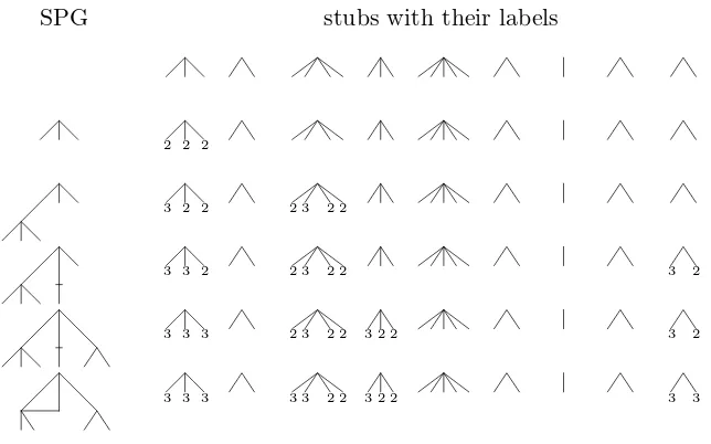
Figure 3: Schematic drawing of the growth of the SPG from the node 1 with N = 9 and the updating of the labels. The stubs without a label are understood to have label 1. The first line shows the N different nodes with their attached stubs. Initially, all stubs have label 1. The growth process starts by choosing the first stub of node 1 whose stubs are labelled by 2 as illustrated in the second line, while all the other stubs maintain the label 1. Next, we uniformly choose a stub with label 1 or 2. In the example in line 3, this is the second stub from node 3, whose stubs are labelled by 2 and the second stub by label 3. The left hand side column visualizes the growth of the SPG by the attachment of stub 2 of node 3 to the first stub of node 1. Once an edge is established the paired stubs are labelled 3. In the next step, again a stub is chosen uniformly out of those with label 1 or 2. In the example in line 4, it is the first stub of the last node that will be attached to the second stub of node 1, the next in sequence to be paired. The last line exhibits the result of creating a cycle when the first stub of node 3 is chosen to be attached to the second stub of node 9 (the last node). This process is continued until there are no more stubs with labels 1 or 2. In this example, we haveZ(1,N)
1 = 3 andZ
(1,N)
2 = 6.
Initially, all stubs are labelled 1. At each stage of the growth of the SPG, we draw uniformly at random from all stubs with labels 1 and 2. After each draw we will update the realization of the SPG according to three categories, which will be labelled 1, 2 and 3. At any stage of the generation of the SPG, the labels have the following meaning:
1. Stubs with label 1 are stubs belonging to a node that is not yet attached to the SPG.
2. Stubs with label 2 are attached to the SPG (because the corresponding node has been chosen), but not yet paired with another stub. These are the ‘free stubs’ mentioned above.
The growth process as depicted in Figure 3 starts by labelling all stubs by 1. Then, because we construct the SPG starting from node 1 we relabel theD1 stubs of node 1 with the label 2. We
note thatZ(1,N)
1 is equal to the number of stubs connected to node 1, and thusZ
(1,N)
1 =D1. We
next identifyZj(1,N) forj >1. Zj(1,N) is obtained by sequentially growing the SPG from the free stubs in generationZ(1,N)
j−1 . When all free stubs in generationj−1 have chosen their connecting
stub, Z(1,N)
j is equal to the number of stubs labelled 2 (i.e., free stubs) attached to the SPG.
Note that not necessarily each stub ofZ(1,N)
j−1 contributes to stubs ofZ
(1,N)
j , because a cycle may
‘swallow’ two free stubs. This is the case when a stub with label 2 is chosen. After the choice of each stub, we update the labels as follows:
1. If the chosen stub has label 1, we connect the present stub to the chosen stub to form an edge and attach the brother stubs of the chosen stub as children. We update the labels as follows. The present and chosen stub melt together to form an edge and both are assigned label 3. All brother stubs receive label 2.
2. When we choose a stub with label 2, which is already connected to the SPG, a self-loop is created if the chosen stub and present stub are brother stubs. If they are not brother stubs, then a cycle is formed. Neither a self-loop nor a cycle changes the distances to the root in the SPG. The updating of the labels solely consists of changing the label of the present and the chosen stubs from 2 to 3.
The above process stops in the jth generation when there are no more free stubs in generation j−1 for the SPG, and then Z(1,N)
j is the number of free stubs at this time. We continue the
above process of drawing stubs until there are no more stubs having label 1 or 2, so that all stubs have label 3. Then, the SPG from node 1 is finalized, and we have generated the shortest path graph as seen from node 1. We have thus obtained the structure of the shortest path graph, and know how many nodes there are at a given distance from node 1.
The above construction will be performed identically from node 2, and we denote the number of free stubs in the SPG of node 2 in generationkby Zk(2,N). This construction is close to being independent, when the generation size is not too large. In particular, it is possible to couple the two SPG growth processes with two independent BP’s. This is described in detail in (14, Section 3). We make essential use of the coupling between the SPG’s and the BP’s, in particular, of (14, Proposition A.3.1) in the appendix. This completes the construction of the SPG’s from both node 1 and 2.
3.3 Bounds on the coupling
We now investigate the relationship between the SPG {Z(i,N)
k } and the BP {Z
(i)
k } with law g.
These results are stated in Proposition 3.1, 3.2 and 3.4. In their statement, we write, fori= 1,2,
Y(i,N)
k = (τ −2)klog(Z
(i,N)
k ∨1) and Y
(i)
k = (τ −2)klog(Z
(i)
k ∨1), (3.1)
where {Zk(1)}k≥1 and {Zk(2)}k≥1 are two independent delayed BP’s with offspring distribution {gj}and where Z1(i) has law {fj}. Then the following proposition shows that the first levels of
Proposition 3.1 (Coupling at fixed time). If F satisfies Assumption 1.1(ii), then for every m fixed, and fori= 1,2, there exist independentdelayed BP’sZ(1),
Z(2), such that
lim
N→∞P(Y
(i,N)
m =Ym(i)) = 1. (3.2)
In words, Proposition 3.1 states that at anyfixedtime, the SPG’s from 1 and 2 can be coupled to two independent BP’s with offspringg, in such a way that the probability that the SPG differs from the BP vanishes when N → ∞.
In the statement of the next proposition, we write, fori= 1,2,
T(i,N)
m =Tm(i,N)(ε) = {k > m: Zm(i,N)
κk−m
≤N1−ε
2
τ−1 }
= {k > m:κkY(i,N)
m ≤
1−ε2
τ −1 logN}, (3.3)
where we recall thatκ= (τ −2)−1. We will see thatZk(i,N) grows super-exponentially withkas long ask∈ T(i,N)
m . More precisely,Zk(i,N) is close to Zm(i,N)κ
k−m
, and thus,T(i,N)
m can be thought
of as the generations for which the generation size is bounded byN1−ε 2
τ−1 . The second main result
of the coupling is the following proposition:
Proposition 3.2 (Super-exponential growth with base Ym(i,N) for large times). If F satisfies
Assumption 1.1(ii), then, for i= 1,2,
(a) P
ε≤Y(i,N)
m ≤ε−1, max k∈Tm(i,N)(ε)
|Yk(i,N)−Y(i,N)
m |> ε3
=oN,m,ε(1), (3.4)
(b) Pε≤Y(i,N)
m ≤ε−1,∃k∈ Tm(i,N)(ε) : Z
(i,N)
k−1 > Z
(i,N)
k
=oN,m,ε(1), (3.5)
Pε≤Y(i,N)
m ≤ε−1,∃k∈ Tm(i,N)(ε) : Z
(i,N)
k > N
1−ε4 τ−1
=oN,m,ε(1), (3.6)
whereoN,m,ε(1)denotes a quantityγN,m,εthat converges to zero when firstN → ∞, thenm→ ∞
and finallyε↓0.
Remark 3.3. Throughout the paper limits will be taken in the above order, i.e., first we send N → ∞, then m→ ∞ and finallyε↓0.
Proposition 3.2 (a), i.e. (3.4), is the main coupling result used in this paper, and says that as long as k ∈ T(i,N)
m (ε), we have that Yk(i,N) is close to Ym(i,N), which, in turn, by Proposition
3.1, is close to Ym(i). This establishes the coupling between the SPG and the BP. Part (b) is a
technical result used in the proof. Equation (3.5) is a convenient result, as it shows that, with high probability, k 7→ Z(i,N)
k is monotonically increasing. Equation (3.6) shows that with high
probability Z(i,N)
k ≤ N
1−ε4
τ−1 for all k ∈ Tm(i,N)(ε), which allows us to bound the number of free
stubs in generation sizes that are inTm(i,N)(ε).
We complete this section with a final coupling result, which shows that for the firstk which is notinT(i,N)
Proposition 3.4(Lower bound onZk(i,N+1)fork+16∈ Tm(i,N)(ε)). LetF satisfy Assumption 1.1(ii).
Then,
P
k∈ T(i,N)
m (ε), k+ 16∈ Tm(i,N)(ε), ε≤Ym(i,N) ≤ε−1, Z
(i,N)
k+1 ≤N
1−ε τ−1
=oN,m,ε(1). (3.7)
Propositions 3.1, 3.2 and 3.4 will be proved in the appendix. In Section 4 and 5, we will prove the main results in Theorems 1.2 and 1.5 subject to Propositions 3.1, 3.2 and 3.4.
4
Proof of Theorems 1.2 and 1.5 for
τ
∈
(2
,
3)
For convenience we combine Theorem 1.2 and Theorem 1.5, in the case that τ ∈ (2,3), in a single theorem that we will prove in this section.
Theorem 4.1. Fixτ ∈(2,3). When Assumption 1.1(ii) holds, then there exist random variables (Rτ,a)a∈(−1,0], such that as N → ∞,
P
HN = 2⌊
log logN
|log(τ −2)|⌋+l
HN <∞
=P(Rτ,aN =l) +o(1), (4.1)
where aN =⌊|log loglog(τ−N2)|⌋ −|log loglog(τ−N2)| ∈(−1,0]. The distribution of(Rτ,a),for a∈(−1,0], is given
by
P(Rτ,a> l) =P
min
s∈Z
(τ−2)−sY(1)+ (τ
−2)s−clY(2)
≤(τ−2)⌈l/2⌉+aY(1)Y(2) >0,
where cl = 1 if l is even, and zero otherwise, and Y(1), Y(2) are two independent copies of the
limit random variable in (1.13).
4.1 Outline of the proof
We start with an outline of the proof. The proof is divided into several key steps proved in 5 subsections, Sections 4.2 - 4.6.
In the first key step of the proof, in Section 4.2, we split the probabilityP(HN > k) into separate
parts depending on the values of Y(i,N)
m = (τ −2)mlog(Zm(i,N)∨1). We prove that
P(HN > k, Ym(1,N)Ym(2,N) = 0) = 1−qm2 +o(1), N → ∞, (4.2)
where 1−qmis the probability that the delayed BP{Zj(1)}j≥1dies at or before themthgeneration.
When mbecomes large, then qm ↑q, where q equals the survival probability of{Zj(1)}j≥1. This
leaves us to determine the contribution to P(HN > k) for the cases whereY
(1,N)
m Ym(2,N) >0. We
further show that for m large enough, and on the event that Ym(i,N) >0, whp, Ym(i,N) ∈[ε, ε−1],
fori = 1,2, where ε >0 is small. We denote the event where Y(i,N)
m ∈[ε, ε−1], fori= 1,2, by
Em,N(ε), and the event where maxk∈T(N)
m (ε)|Y
(i,N)
k −Y
(i,N)
m | ≤ ε3 for i= 1,2 by Fm,N(ε). The
eventsEm,N(ε) andFm,N(ε) are shown to occurwhp, forFm,N(ε) this follows from Proposition
The second key step in the proof, in Section 4.3, is to obtain an asymptotic formula forP({HN>
j−1}. Basically this follows from the multiplication rule. The identity (4.3) is established in (4.32).
Proposition 3.2, it implies thatwhp
Z(1,N)
In turn, these bounds allow us to use Proposition 3.2(a). Combining (4.3) and (4.4), we establish in Corollary 4.10, that for alll and with
kN = 2
In the final key step, in Sections 4.5 and 4.6, the minimum occurring in (4.6), with the approx-imations Y(1,N)
k1+1 ≈Y (1,N)
m and Yk(2N,N−)k1 ≈Ym(2,N), is analyzed. The main idea in this analysis is as
follows. With the above approximations, the right side of (4.6) can be rewritten as
E The minimum appearing in the exponent of (4.7) is then rewritten (see (4.73) and (4.75)) as
Here it will become apparent that the bounds 12 ≤λN(k) ≤4k are sufficient. The expectation
of the indicator of this event leads to the probability
P
min
t∈Z(κ
tY(1)+κcl−tY(2))
≤κaN−⌈l/2⌉, Y(1)Y(2)>0
,
withaNandclas defined in Theorem 4.1. We complete the proof by showing that conditioning on
the event that 1 and 2 are connected is asymptotically equivalent to conditioning onY(1)Y(2)>0.
Remark 4.2. In the course of the proof, we will see that it is not necessary that the degrees of the nodes are i.i.d. In fact, in the proof below, we need that Propositions 3.1–3.4 are valid, as well as thatLN is concentrated around its mean µN. In Remark A.1.5 in the appendix, we will
investigate what is needed in the proof of Propositions 3.1– 3.4. In particular, the proof applies also to some instances of the configuration model where the number of nodes with degree k is deterministic for eachk, when we investigate the distance between two uniformlychosen nodes.
We now go through the details of the proof.
4.2 A priory bounds on Y(i,N)
m
We wish to compute the probabilityP(HN > k). To do so, we split P(HN > k) as
P(HN > k) =P(HN> k, Ym(1,N)Ym(2,N) = 0) +P(HN> k, Ym(1,N)Ym(2,N) >0). (4.8)
We will now prove two lemmas, and use these to compute the first term in the right-hand side of (4.8).
Lemma 4.3. For any m fixed,
lim
N→∞P(Y
(1,N)
m Ym(2,N)= 0) = 1−q2m,
where
qm =P(Ym(1) >0).
Proof. The proof is immediate from Proposition 3.1 and the independence ofYm(1)andYm(2).
The following lemma shows that the probability thatHN ≤mconverges to zero for anyfixedm:
Lemma 4.4. For any m fixed,
lim
N→∞P(HN ≤m) = 0.
Proof. As observed above Theorem 1.2, by exchangeability of the nodes{1,2, . . . , N},
P(HN ≤m) =P(HeN ≤m), (4.9)
whereHeN is the hopcount between node 1 and a uniformly chosen node unequal to 1. We split,
for any 0< δ <1,
P(HeN ≤m) =P(HeN ≤m,
X
j≤m
Z(1,N)
j ≤Nδ) +P(HeN ≤m,
X
j≤m
Z(1,N)
The number of nodes at distance at mostmfrom node 1 is bounded from above byPj≤mZj(1,N).
Therefore, the first term in (4.10) is o(1), as required. We will proceed with the second term in (4.10). By Proposition 3.1, whp, we have that Yj(1,N) = Yj(1) for all j ≤ m. Therefore, we
However, when m is fixed, the random variable Pj≤mZj(1) is finite with probability 1, and therefore,
This completes the proof of Lemma 4.4.
We now use Lemmas 4.3 and 4.4 to compute the first term in (4.8). We split
P(HN > k, Y
Using Lemma 4.4, we conclude that
Corollary 4.5. For every m fixed, and each k∈N, possibly depending on N,
and similarly for the second probability. The remainder of the proof of the lemma follows because Y(i)
m →d Y(i) asm → ∞, and because conditionally onY(i) >0 the random variable Y(i) admits
a density.
Write
Em,N =Em,N(ε) ={Y
(i,N)
m ∈[ε, ε−1], i= 1,2}, (4.15)
Fm,N =Fm,N(ε) =
max
k∈Tm(N)(ε)
|Y(i,N)
k −Y
(i,N)
m | ≤ε3, i= 1,2 . (4.16)
As a consequence of Lemma 4.6, we obtain that
P(Em,c N∩ {Y
(1,N)
m Ym(2,N)>0}) =oN,m,ε(1), (4.17)
so that
P(HN > k, Ym(1,N)Ym(2,N)>0) =P({HN > k} ∩Em,N) +oN,m,ε(1). (4.18)
In the sequel, we compute
P({HN > k} ∩Em,N), (4.19)
and often we will make use of the fact that by Proposition 3.2,
P(Em,N∩Fm,c N) =oN,m,ε(1). (4.20)
4.3 Asymptotics of P({HN > k} ∩Em,N)
We next give a representation ofP({HN > k} ∩Em,N). In order to do so, we writeQ
(i,j)
Z , where
i, j≥0, for the conditional probability given {Z(1,N)
s }is=1 and {Zs(2,N)}js=1 (where, for j= 0, we
condition only on {Z(1,N)
s }is=1), and E
(i,j)
Z for its conditional expectation. Furthermore, we say
that a random variable k1 is Zm-measurable if k1 is measurable with respect to the σ-algebra
generated by{Z(1,N)
s }ms=1 and {Zs(2,N)}ms=1. The main rewrite is now in the following lemma:
Lemma 4.7. For k≥2m−1,
P({HN > k} ∩Em,N) =E
h
1Em,NQ
(m,m)
Z (HN >2m−1)Pm(k, k1)
i
, (4.21)
where, for anyZm-measurable k1, with m≤k1 ≤(k−1)/2,
Pm(k, k1) = 2k1 Y
i=2m
Q(⌊Zi/2⌋+1,⌈i/2⌉)(HN > i|HN > i−1) (4.22)
×
k−Y2k1
i=1
Q(k1+1,k1+i)
Z (HN>2k1+i|HN >2k1+i−1).
Proof. We start by conditioning on {Z(1,N)
s }ms=1 and {Z
(2,N)
s }ms=1, and note that 1Em,N is Zm
-measurable, so that we obtain, fork≥2m−1,
P({HN > k} ∩Em,N) =E
h
1Em,NQ
(m,m)
Z (HN > k)
i
(4.23)
=Eh1Em,NQ
(m,m)
Z (HN >2m−1)Q
(m,m)
Z (HN > k|HN >2m−1)
i
Moreover, fori, j such that i+j≤k,
Q(Zi,j)(HN > k|HN > i+j−1) (4.24)
=E(Zi,j)Q(Zi,j+1)(HN> k|HN > i+j−1)
=E(Zi,j)Q(Zi,j+1)(HN > i+j|HN > i+j−1)Q
(i,j+1)
Z (HN > k|HN > i+j)
,
and, similarly,
Q(Zi,j)(HN > k|HN > i+j−1) (4.25)
=E(Zi,j)Q(Zi+1,j)(HN > i+j|HN > i+j−1)Q
(i+1,j)
Z (HN > k|HN > i+j)
.
In particular, we obtain, fork >2m−1,
Q(Zm,m)(HN > k|HN >2m−1) =E
(m,m)
Z
h
Q(Zm+1,m)(HN >2m|HN >2m−1) (4.26)
×Q(Zm+1,m)(HN > k|HN >2m)
i
,
so that, using thatEm,N isZm-measurable and thatE[EZ(m,m)[X]] =E[X] for any random variable
X,
P({HN > k} ∩Em,N) (4.27)
=E
h
1Em,NQ
(m,m)
Z (HN>2m−1)Q
(m+1,m)
Z (HN >2m|HN >2m−1)Q
(m+1,m)
Z (HN > k|HN >2m)
i
.
We now compute the conditional probability by repeatedly applying (4.24) and (4.25), increasing iorj as follows. Fori+j≤2k1, we will increaseiand j in turn by 1, and for 2k1 < i+j≤k,
we will only increase the second componentj. This leads to
Q(Zm,m)(HN > k|HN >2m−1) =E
(m,m)
Z
h Y2k1
i=2m
Q(⌊Zi/2⌋+1,⌈i/2⌉)(HN > i|HN > i−1) (4.28)
×
k−Y2k1
j=1
Q(k1+1,k1+j)
Z (HN >2k1+j|HN >2k1+j−1)
i
=E(Zm,m)[Pm(k, k1)],
were we used that we can move the expectationsE(Zi,j) outside, as in (4.27), so that these do not appear in the final formula. Therefore, from (4.23), (4.28), and since 1Em,N and Q
(m,m)
Z (HN >
2m−1) areZm-measurable,
P({HN > k} ∩Em,N) =E
h
1Em,NQ
(m,m)
Z (HN >2m−1)E
(m,m)
Z [Pm(k, k1)]
i
=E
h
E(Zm,m)[1Em,NQ
(m,m)
Z (HN >2m−1)Pm(k, k1)]
i
=Eh1Em,NQ
(m,m)
Z (HN >2m−1)Pm(k, k1)
i
. (4.29)
We note that we can omit the termQ(Zm,m)(HN >2m−1) in (4.21) by introducing a small error
term. Indeed, we can write
Q(Zm,m)(HN >2m−1) = 1−Q
(m,m)
Z (HN ≤2m−1). (4.30)
Bounding 1Em,NPm(k, k1)≤ 1, the contribution to (4.21) due to the second term in the
right-hand side of (4.30) is according to Lemma 4.4 bounded by
EhQ(Zm,m)(HN ≤2m−1)
i
=P(HN ≤2m−1) =oN(1). (4.31)
We conclude from (4.20), (4.21), and (4.31), that
P({HN > k} ∩Em,N) =E
h
1Em,N∩Fm,NPm(k, k1)
i
+oN,m,ε(1). (4.32)
We continue with (4.32) by bounding the conditional probabilities inPm(k, k1) defined in (4.22).
Lemma 4.8. For all integers i, j≥0,
exp
(
−4Z
(1,N)
i+1 Z
(2,N)
j
LN
)
≤Q(Zi+1,j)(HN > i+j|HN > i+j−1)≤exp
(
−Z
(1,N)
i+1 Z
(2,N)
j
2LN
)
. (4.33)
The upper bound is always valid, the lower bound is valid whenever
i+1
X
s=1
Z(1,N)
s + j
X
s=1
Z(2,N)
s ≤
LN
4 . (4.34)
Proof. We start with the upper bound. We fix two sets of n1 and n2 stubs, and will be
interested in the probability that none of then1 stubs are connected to then2 stubs. We order
then1 stubs in an arbitrary way, and connect the stubs iteratively to other stubs. Note that we
must connect at least ⌈n1/2⌉ stubs, since any stub that is being connected removes at most 2
stubs from the total ofn1 stubs. The numbern1/2 is reached forn1 even precisely when all the
n1 stubs are connected with each other. Therefore, we obtain that the probability that then1
stubs are not connected to the n2 stubs is bounded from above by
⌈nY1/2⌉
t=1
1− n2 LN−2t+ 1
≤ ⌈nY1/2⌉
t=1
1− n2 LN
. (4.35)
Using the inequality 1−x ≤e−x, x ≥ 0, we obtain that the probability that the n1 stubs are
not connected to then2 stubs is bounded from above by
e−⌈n1/2⌉LNn2
≤e−
n1n2
2LN. (4.36)
Applying the above bound ton1 =Zi(1+1,N) and n2 =Zj(2,N), and noting that the probability that
HN > i+j given that HN > i+j−1 is bounded from above by the probability that none of
theZ(1,N)
i+1 stubs are connected to theZ
(2,N)
j stubs leads to the upper bound in (4.33).
We again fix two sets ofn1 andn2 stubs, and are again interested in the probability that none of
we assume that in each step there remain to be at leastLstubs available. We order then1 stubs
in an arbitrary way, and connect the stubs iteratively to other stubs. We obtain a lower bound by further requiring that then1 stubs do not connect to each other. Therefore, the probability
that then1 stubs are not connected to then2 stubs is bounded below by
n1
then the probability that then1 stubs are not connected to then2 stubs when there are still at
leastL stubs available is bounded below by
n1
i+1 stubs are connected to the Z
(2,N)
j stubs. We will assume that (4.34) holds. We have that
L = LN −2
(4.34). Thus, we are allowed to use the bound in (4.38). This leads to
Q(Zi+1,j)(HN > i+j|HN > i+j−1) ≥exp
which completes the proof of Lemma 4.8.
4.4 The main contribution to P({HN > k} ∩Em,N)
We rewrite the expression in (4.32) in a more convenient form, using Lemma 4.8. We derive an upper and a lower bound. For the upper bound, we bound all terms appearing on the right-hand side of (4.22) by 1, except for the term Q(k1+1,k−k1)
To derive the lower bound, we next assume that
so that (4.34) is satisfied for all iin (4.22). We write, recalling (3.3),
it follows from Proposition 3.2 that ifk1 ∈ B(1)N (ε, k), that then, with probability converging to
1 as firstN → ∞and then m→ ∞, Therefore, by Lemma 4.7, and using the above bounds for each of the in totalk−2m+ 1 terms, we obtain that whenk1 ∈ BN(1)(ε, k)6=∅, and with probability 1−oN,m,ε(1),
We next use the symmetry for the nodes 1 and 2. Denote
We defineBN(ε, k) =B
(1)
N (ε, k)∪ B
(2)
N (ε, k), which is equal to
BN(ε, k) =
n
m≤l≤k−1−m: l+ 1∈ T(1,N)
m (ε), k−l∈ Tm(2,N)(ε)
o
. (4.51)
We can summarize the obtained results by writing that with probability 1−oN,m,ε(1), and when
BN(ε, k)6=∅, we have
Pm(k, k1) = exp
−λN
Zk(11,N+1)Zk(2−,Nk)1 LN
, (4.52)
for all k1 ∈ BN(ε, k), whereλN =λN(k) satisfies
1
2 ≤λN(k)≤4k. (4.53)
Relation (4.52) is true for anyk1 ∈ BN(ε, k). However, our coupling fails when Z
(1,N)
k1+1 or Z (2,N)
k−k1
grows too large, since we can only coupleZj(i,N) with ˆZj(i,N) up to the point whereZj(i,N)≤N1−ε 2
τ−1 .
Therefore, we next take the maximal value over k1 ∈ BN(ε, k) to arrive at the fact that, with
probability 1−oN,m,ε(1), on the event thatBN(ε, k)6=∅,
Pm(k, k1) = max
k1∈BN(ε,k)
exp−λN
Z(1,N)
k1+1Z (2,N)
k−k1 LN
= expn−λN min
k1∈BN(ε,k)
Z(1,N)
k1+1Z (2,N)
k−k1 LN
o
. (4.54)
From here on we take k=kN as in (4.5) withl a fixed integer.
In Section 5, we prove the following lemma that shows that, apart from an event of probability 1−oN,m,ε(1), we may assume thatBN(ε, kN)6=∅:
Lemma 4.9. For all l, with kN as in (4.5),
lim sup
ε↓0
lim sup
m→∞ lim supN→∞
P({HN> kN} ∩Em,N∩ {BN(ε, kN) =∅}) = 0.
From now on, we will abbreviate BN = BN(ε, kN). Using (4.32), (4.54) and Lemma 4.9, we
conclude that,
Corollary 4.10. For all l, with kN as in (4.5),
P {HN > kN} ∩Em,N
=E
h
1Em,N∩Fm,Nexp
n
−λN min
k1∈BN
Z(1,N)
k1+1Z (2,N)
kN−k1 LN
oi
+oN,m,ε(1),
where
1
2 ≤λN(kN)≤4kN.
4.5 Application of the coupling results
Lemma 4.11. Suppose that y1 > y2 >0, and κ= (τ −2)−1 >1. Fix an integer n, satisfying
where round(x) isx rounded off to the nearest integer. In particular,
max
Proof. Consider, for real-valued t∈[0, n], the function
ψ(t) =κty1+κn−ty2.
Then,
ψ′(t) = (κty1−κn−ty2) logκ, ψ′′(t) = (κty1+κn−ty2) log2κ.
In particular,ψ′′(t)>0, so that the function ψ is strictly convex. The unique minimum of ψis attained at ˆt, satisfyingψ′(ˆt) = 0, i.e.,
where we rewrite, using (4.51) and (3.3),
To abbreviate the notation, we will write, for i= 1,2,
Y(i,N)
On the complement Hc
m,N, the minimum over 0 ≤ k1 ≤ kN−1 of κk1+1Y
Therefore, in the remainder of the proof, we assume thatHm,N holds.
Lemma 4.12. With probability exceeding1−oN,m,ε(1),
Proof. We start with (4.61), the proof of (4.62) is similar, and, in fact, slightly simpler, and is
Moreover, by (4.63), we have that
1≤ x
whenε >0 is sufficiently small. We claim that if (note the difference with (4.67)),
x=κt∗Y(1,N)
so that the first bound in (4.57) is satisfied. The second bound is satisfied, since
We conclude that, in order to show that (4.61) holds with error at most oN,m,ε(1), we have to
show that the probability of the intersection of the events {HN > kN} and
Em,N=Em,N(ε) =
n
∃t: 1−ε
τ −1logN < κ
tY(1,N)
m,+ ≤
1 +ε
τ −1logN, (4.71) κtY(1,N)
m,+ +κn−tY
(2,N)
m,+ ≤(1 +ε) logN
o
,
is of order oN,m,ε(1). This is contained in Lemma 4.13 below.
Lemma 4.13. ForkN as in (4.5),
lim sup
ε↓0
lim sup
m→∞ lim supN→∞
P(Em,N(ε)∩ Em,N(ε)∩ {HN > kN}) = 0.
The proof of Lemma 4.13 is deferred to Section 5. From (4.56), Lemmas 4.12 and 4.13, we finally arrive at
P {HN > kN} ∩Em,N
(4.72)
≤Eh1Em,Nexp
n
−λNexp
h
min
0≤k1<kN
κk1+1Y(1,N)
m,− +κkN−k1Ym,(2,N−)
−logLN
ioi
+oN,m,ε(1),
and at a similar lower bound whereYm,(i,N−) is replaced byYm,(i,N+). Note that on the right-hand side of (4.72), we have replaced the intersection of 1Em,N∩Fm,N by 1Em,N, which is allowed, because
of (4.20).
4.6 Evaluating the limit
The final argument starts from (4.72) and the similar lower bound, and consists of lettingN → ∞ and then m → ∞. The argument has to be performed with Y(i,N)
m,+ and Ym,(i,N−) separately, after
which we let ε↓0. Since the precise value ofεplays no role in the derivation, we only give the derivation for ε= 0. Observe that
min
0≤k1<kN
(κk1+1Y(1,N)
m +κkN−k1Ym(2,N))−logLN
=κ⌈kN/2⌉ min
0≤k1<kN
κk1+1−⌈kN/2⌉Y(1,N)
m +κ⌊kN/2⌋−k1Ym(2,N)−κ−⌈kN/2⌉logLN
=κ⌈kN/2⌉ min
−⌈kN/2⌉+1≤t<⌊kN/2⌋+1
(κtY(1,N)
m +κcl−tYm(2,N)−κ−⌈kN/2⌉logLN), (4.73)
wheret=k1+ 1− ⌈kN/2⌉,ckN =cl =⌊l/2⌋ − ⌈l/2⌉+ 1 =1{l is even}. We further rewrite, using
the definition ofaN in Theorem 4.1,
κ−⌈kN/2⌉logL N=κ
log logN
logκ −⌊
log logN
logκ ⌋−⌈l/2⌉logLN
logN =κ
−aN−⌈l/2⌉logLN
logN . (4.74)
Calculating, for Y(i,N)
m ∈ [ε, ε−1], the minimum of κtYm(1,N) +κcl−tYm(2,N), over all t ∈ Z, we
conclude that the argument of the minimum is contained in the interval [12,12+ log(ε2)/2 logκ].
Hence from Lemma 4.11, for N → ∞,n=cl∈ {0,1} and on the eventEm,N,
min
−⌈kN/2⌉+1≤t≤⌊kN/2⌋
(κtY(1,N)
m +κcl−tYm(2,N)) = min t∈Z(κ
tY(1,N)
We define
The upper and lower bound in (4.72) now yield:
Eh1Em,Nexp
The split (4.78) is correct since (using the abbreviation expW for exp−λNeκ
⌈kN /2⌉W
Finally, we boundKN by
KN ≤P(FeNc ∩Ge
c
N∩Em,N), (4.87)
Lemma 4.14. For all l,
lim sup
ε↓0
lim sup
m→∞
lim sup
N→∞
P FeN(l, ε)c ∩GeN(l, ε)c∩Em,N(ε)
= 0.
The conclusion from (4.77)-(4.87) is that:
P({HN > kN} ∩Em,N) =P(GeN∩Em,N) +oN,m,ε(1). (4.88)
To compute the main termP(GeN∩Em,N), we define
Ul= min t∈Z(κ
tY(1)+κcl−tY(2)), (4.89)
and we will show that
Lemma 4.15.
P(GeN∩Em,N) =P Ul−κ−aN−⌈l/2⌉<0, Y
(1)Y(2)>0+o
N,m,ε(1). (4.90)
Proof. From the definition of GeN,
e
GN∩Em,N =
n
min
t∈Z(κ
tY(1,N)
m +κcl−tYm(2,N))−κ−aN−⌈l/2⌉
logUN
logN <−ε, Y (i,N)
m ∈[ε, ε−1]
o
. (4.91)
By Proposition 3.1 and the fact thatLN =µN(1 +o(1)),
P(GeN∩Em,N)−P
min
t∈Z(κ
tY(1)
m +κcl−tYm(2))−κ−aN−⌈l/2⌉<−ε, Ym(i) ∈[ε, ε−1]
=oN,m,ε(1). (4.92)
SinceYm(i) converges toY(i) almost surely, asm→ ∞, sups≥m|Y
(i)
s −Y(i)|converges to 0 a.s. as
m→ ∞. Therefore,
P(GeN∩Em,N)−P
Ul−κ−aN−⌈l/2⌉<−ε, Y(i)∈[ε, ε−1]
=oN,m,ε(1), (4.93)
Moreover, sinceY(1) has a density on (0,∞) and an atom at 0 (see (8)),
P(Y(1)
6∈[ε, ε−1], Y(1)>0) =o(1), asε
↓0.
Recall from Section 3.1 that for any l fixed, and conditionally on Y(1)Y(2) > 0, the random
variable Ul has a density. We denote this density by f2 and the distribution function by F2.
Also,κ−aN−⌈l/2⌉∈I
l = [κ−⌈l/2⌉, κ−⌈l/2⌉+1]. Then,
P
−ε≤Ul−κ−aN−⌈l/2⌉<0
≤sup
a∈Il
[F2(a)−F2(a−ε)]. (4.94)
The function F2 is continuous on Il, so that in fact F2 is uniformly continuous on Il, and we
conclude that
lim sup
ε↓0
sup
a∈Il
[F2(a)−F2(a−ε)] = 0. (4.95)
This establishes (4.90).