www.elsevier.nl / locate / econbase
Learning to make risk neutral choices in a symmetric world
a b ,*
Stefano DellaVigna , Marco LiCalzi a
Department of Economics, Harvard University, Littaver Center, Cambridge, MA 02138-3001, USA b
Department of Applied Mathematics, University of Venice, Dorsoduro 3825 /E, I-30123 Venezia, Italy Received 18 June 1998; received in revised form 30 November 1999; accepted 13 January 2000
Abstract
Given their reference point, most people tend to be risk averse over gains and risk seeking over losses. Therefore, they exhibit a dual risk attitude which is reference dependent. This paper considers an adaptive process for choice under risk such that, in spite of a permanent short-run dual risk attitude, the agent eventually learns to make risk neutral choices. The adaptive process is based on an aspiration level, endogenously adjusted over time in the direction of the actually experienced payoff. 2001 Elsevier Science B.V. All rights reserved.
Keywords: Risk attitude; Reference point; Aspiration level; Target; Prospect theory; Reflection effect JEL classification: D81; D83
1. Introduction
Among economists, the most common assumption about choice behavior under risk is that people maximize expected utility. The second most common assumption is that they are risk averse. Serious difficulties in reconciling this second hypothesis with the empirical evidence have been known since Friedman and Savage (1948). As a way to deal with those, Markowitz (1952) suggested that the utility function might shift depending on the current wealth.
This long forgotten intuition was revived by Kahneman and Tversky (1979) and Fishburn and Kochenberger (1979). They showed how the empirical evidence supports a model where the utility function of an agent is based on a reference point such as her current level of wealth. While people may focus on different reference points, see Heath
*Corresponding author. Tel.:139-041-790925; fax:139-041-5221756. E-mail address: [email protected] (M. LiCalzi).
et al. (1999), most agents tend to exhibit what Kahneman and Tversky (1979) called the reflection effect: they are risk averse in the gains and risk seeking in the losses with respect to their reference point. A variety of studies and psychological explanations surveyed in Kahneman et al. (1991) has established that there is a dual risk attitude which depends on the reference point.
The risk attitude, therefore, is not an intrinsic feature of the choice behavior of an agent. Whatever affects the reference point may determine the risk attitude. Depending on the context and her past experiences, the same agent might seek or avert risk and henceforth make different choices over the same set of lotteries. This compels economics to confront two questions: (i) whether her choice behavior may converge (and hence become predictable) in the long run; (ii) which kind of risk attitude would eventually emerge?
March (1996) approaches the second question showing that a stimulus-response model of experiential learning tends to generate a dual risk attitude in a simple bandit problem. While he considers possible generalizations, he explicitly warns that ‘‘adaptive aspirations present a more complicated problem’’ (p. 317). This paper studies a model of aspiration-based learning over a known domain of symmetrically distributed payoffs where, while maintaining reference-dependent preferences in the short run, the agent eventually learns to choose a lottery which maximizes expected value. Our results answer the first question in the positive and suggest an important distinction in the second one: even if the agent has a dual risk attitude, this does not rule out her making risk-neutral choices in the long run.
The following outline gives the essential features of our model. The agent repeatedly faces a choice problem over monetary lotteries that are symmetrically distributed. Her reference point is based on an aspiration level which acts as a target. At each period, the agent picks a lottery that maximizes the probability of meeting her current target. Right after, she plays the lottery and adjusts her reference point for the next period in the direction of the actually experienced payoff. In the long-run, the reference point settles down to a specific value and her choice behavior converges to maximization of the expected value. However, at each period the agent maintains a dual risk attitude which never withers away: therefore, learning to make risk neutral choices takes place without the agent learning to be risk neutral.
The crucial idea for this result is simple: since preferences (and hence choices) depend on the reference point, long-run convergence of the choice behavior follows from the convergence of the reference point. Our model, however, has other features as well. We endogenize the reference point and make it depend on the outcome of the past choices. A simple rule of aspiration adaptation provides the link between the evolution of long-run preferences and the short-run choice behavior. Moreover, we model short-run preferences using an approach which is independent of the expected utility hypothesis, while still consistent with it. This provides a simple generalization of the reflection effect to the case of lotteries which simultaneously involve gains and losses.
selects some strategies resulting in an outcome that affects players’ beliefs in the next period. Against a fixed behavior rule, beliefs evolve endogenously. Thus, convergence to equilibrium behavior follows from convergence to equilibrium beliefs.
Here, we postulate that the behavior rule is target-based maximization. Combined with the agent’s current reference point, this rule selects a lottery resulting in an outcome that affects her target for the next period. Against a fixed behavior rule, the reference point evolves endogenously. Convergence to a risk neutral choice follows from convergence of the reference point to the ‘right’ level.
The importance of maintaining the ‘right’ aspiration level is stressed in Gilboa and Schmeidler (1996). They show that a case-based decision maker who follows an appropriate adjustment rule for his aspiration level learns to maximize expected utility in a bandit problem. As in our model, they postulate that in each period the agent follows a
¨
deterministic rule of maximization. Borgers and Sarin (1996), instead, study a model where the agent’s choice rule is stochastic. At each period, the agent raises (or lowers) the probability to choose the lottery just selected according to whether its outcome met (or not) her current target. As in our model, the aspiration level is adjusted in the direction of the experienced payoffs. However, since the choice rule introduces probability matching effects, choice behavior usually fails to converge to expected value maximization.
Both of these papers are concerned with choice behavior. Rubin and Paul (1979) and Robson (1996), instead, discuss the formation of individual risk attitudes from an evolutionary viewpoint. Measuring success by the expected number of offsprings, they investigate which kinds of risk attitudes are more likely to emerge. While they suggest reasons for risk seeking over losses by younger males, this approach has not yet been able to fully account for reference-dependent preferences. Dekel et al. (1998) go further and study the endogenous determination of preferences in evolutionary games, but provide no specific results on the evolution of risk attitudes.
2. The short-run model
This section describes our target-based model for the short-run choice behavior. The long-run dynamics of our model is studied in the next section. For the sake of readability, we relegate most proofs and a few auxiliary results to Appendix A.
2.1. Preliminaries
The agent faces a finite (nonempty) set+of monetary lotteries out of which she must choose one. With no loss of generality, we assume that probabilities are exogenously given. All the lotteries in + have finite variance. We denote by m ands respectively
i i
the expected value and the standard deviation of a lottery X in +. We write X|F to i
denote that F is the cumulative distribution function (for short, c.d.f.) of X.
F(m)51 / 2. Therefore, we define m as the median of a symmetrically distributed X. Note that our definition implies that m is unique even if the set of xs such that
F(x)51 / 2 is not a singleton. Moreover, if the expected value of X is finite, this is equal to m. Therefore, for a symmetrically distributed lottery X, we denote both the median and the expected value by m.
We suppose that all the lotteries in + are symmetrically distributed and that their c.d.f.s are absolutely continuous with full support on R. This restrictive assumption is maintained throughout the paper. For the mere purpose of exemplification, we will occasionally assume that the lotteries in + are normally distributed.
2.2. Target-based ranking
In order to make her choice, the agent must rank the lotteries. We assume that she follows the target-based procedure described in Bordley and LiCalzi (2000). Let V denotes the agent’s target, representing her aspiration level. The agent is interested in maximizing the probability of meeting her target. Therefore, she ranks a lottery X in+ by the index w(X )5P(X$V ); that is, by the probability that X meets her target. To
allow for the case where the agent does not know exactly her aspiration level, we assume that V is a random variable with a subjective distribution stochastically independent of+. Therefore, the agent ranks X|F by the index
w(X )5P(X$V )5
E
P(x$V ) dF(x). (1)Given that the agent relies on an uncertain target to rank the available lotteries, we need to formulate some assumptions on the distribution of her aspiration level. In a world where all lotteries are symmetrically distributed, the most natural hypothesis is that the agent’s target V is also symmetrically distributed. We refer to the situation where both the lotteries in + and the target are symmetrically distributed as a ‘symmetric world’. When lotteries and target are taken to be normally distributed, we speak of a ‘normal world’.
An agent using the target-based procedure may not be sure about what her aspiration level V should be. Unless this target is precisely known to her, it is not clear how the agent should decide to code a specific outcome as a gain or as a loss. According to prospect theory, the agent sets a reference point n inR and classifies an outcome as a gain or as a loss according to its being higher or lower than n.
Therefore, we need some assumptions to relate the target V with the reference pointn. If the target is degenerate, it is reasonable to expect it to coincide with the reference point. More generally, a natural assumption might be to letnbe the mode of the target. This matches the intuition that in many cases the agent is likely to anchor her perceptions to the modal outcome. However, the mode of V may not be unique and there may be reasons to prefer other statistics. For instance, one might suggest to let the reference point be some central statistics like the expected value or the median of V. Note though that these two statistics usually differ for non-symmetric distributions.
symmetrically distributed, its expected value and its median have the same value. Moreover, if the distribution of the target is unimodal, the mode is unique and is also equal to the expected value. Given that any of these three statistics can claim to be a prominent anchor and that they all coincide, we let the reference point be the expected value n of the aspiration level V. Note that the assumption of a unimodal target is not part of our definition of a symmetric world: except for the next section, this assumption is not used in the rest of the paper.
2.3. Dual risk attitude
This section shows that, in a symmetric world where the distribution of the target is unimodal, the agent exhibits a dual risk attitude centered around her reference point. This matches the compelling evidence that decision makers tend to be risk averse with respect to gains over their reference point and risk seeking with respect to losses.
We illustrate the point with an example based on a ‘normal’ world. Assume temporarily that all the lotteries in + are normally distributed with strictly positive variances and, by analogy, that the target is also normally distributed with expected valuen and standard deviation s.0; for short, we write V|N(n, s). By Theorem A.1 in Appendix A,
m 2 n ]]] P(X$V )5F
S
Œ
]]2 2D
,s 1s
whereF is the c.d.f. of a standard normal.
Given a lottery X with expected valuem, denote by c(X ) the certainty equivalent of X. An agent is said to be risk averse over X if her certainty equivalent c(X )#m; correspondingly, she is risk seeking if c(X )$m and risk neutral if equality holds. In a normal world, the certainty equivalent exists and is unique for any lottery. If the agent follows the target-based ranking procedure, Theorem A.2 in the Appendix shows that her certainty equivalent for X can be written as a convex combination of m andn:
c(X )5am 1(12a)n, (2)
where of coursea is in [0, 1]. Therefore, the agent is risk averse (respectively, neutral or seeking) over all lotteries that have a higher (equal or lower) expected valuem than her reference pointn. To put it differently, she tends to be more cautious when she expects (on average) to meet her target.
We think that this result fits the spirit of prospect theory. However, we must point out that this is not the reflection effect studied by Kahneman and Tversky (1979). They confronted subjects with pairs of lotteries yielding only positive payoffs and most choices exhibited risk aversion; then they changed positive with negative payoffs and several people switched to risk seeking behavior. Each lottery they examined was on just one side of the reference point. In our normal world, instead, the lotteries in+ have full support and therefore none of them offers only gains (or losses).
Asm↓n, her ‘positive’ perception of X becomes weaker and weaker until m 5 n. At this point, the lottery X is as likely to yield outcomes above the reference point as below and the agent perceives it as ‘balanced’, so that she exhibits risk neutrality. For m , n, the lottery becomes mostly ‘negative’ and the agent turns to a risk seeking behavior.
There is another subtler difference between our approach and Kahneman and Tversky (1979). We postulate target-based ranking as a behavior rule and use this assumption to deduce that the agent will exhibit a dual risk attitude. Kahneman and Tversky (1979), instead, start off from the empirical evidence about dual risk attitudes and show that it may be accounted for by a reflection effect in the utility function. In a sense, while we are trying to suggest an explanatory mechanism, they simply strive to obtain a robust description of the empirical evidence; see Gigerenzer (1996). Moreover, they build their descriptive model by amending the expected utility model (to a significant extent) while we abstract from it.
Our model for a dual risk attitude essentially carries over to a symmetric world, provided that the distribution of the target is unimodal. The whole argument rests on the validity of Eq. (2) in a normal world. When trying to extend the equation to a symmetric world, one runs into the technical difficulty that the existence of the certainty equivalent for any lottery X cannot be guaranteed without further regularity assumptions. Theorem A.4 in Appendix A proves that Eq. (2) holds whenever the certainty equivalent of X exists and V has a unimodal distribution. Thus, if we base the definition of risk attitude on the certainty equivalent, unimodality of the target implies that the dual risk attitude holds in a symmetric world as well.
2.4. The relationship with expected utility
It is instructive to consider how our agent would look like to someone trying to interpret her choice behavior in view of the expected utility model. Maybe surprisingly, her target-based ranking procedure is both mathematically and observationally equiva-lent to the expected utility model. This is shown by Castagnoli and LiCalzi (1996) in von Neumann and Morgenstern’s setting and by Bordley and LiCalzi (2000) in Savage’s framework. For our purposes here, it suffices to note that the choice behavior associated with (1) is compatible with the expected utility model provided that we interpret P(x$V ) as the utility of the outcome x; that is, if we let U(x)5P(x$V ). Accordingly,
we denote the c.d.f. of the uncertain target V by U and write V|U.
To illustrate this point, we assume a normal world where the target V is normally distributed with expected valuen and standard deviation s.0; then P(x$V )5Ff(x2 n) /s . An agent that maximizes the probability to meet the target V would rank allg
lotteries as if she is maximizing the expected value of the utility function U(x)5Ff(x2 n) /s . Either approach makes exactly the same predictions.g
For instance, note thatFf(x2n) /s is concave for xg $nand convex otherwise. In the language of expected utility, we say that the utility function U(x) is S-shaped around n. In the target-based language, we say that the distribution of the target is unimodal. In either case, this characteristic curvature generates a reflection effect around the reference point n.
raises an important modelling issue: why the second and not the first one? There are two independent reasons for this choice. First, the target-based procedure offers a more plausible account of how reference dependence may come into place in the short run. Second, it suggests a natural way to aggregate many short-run choices into a single long-run process. For other modelling advantages of a target-based language see LiCalzi (2000). We argue here for the first claim and defer the discussion of the second one to Section 3.4.
There is a tendency to confound the assumption that the expected utility model represents the agent’s preferences with the claim that the agent actually uses expected utility to find out what she likes better. The first viewpoint is descriptive: the purpose of a theory is to describe behavior, not to explain it. Following this viewpoint, it is immaterial which model we adopt provided that it shares the same descriptive accuracy of its competitors. Both an S-shaped utility function and a unimodal target generate the reflection effect. Therefore, they are equally good and equally bad.
The second viewpoint is closer to looking for an explanation of the observed behavior. An S-shaped utility function does not explain much. The target-based procedure suggests a mechanism which may be the cause behind the reflection effect. Suppose that the agent is not sure about her target and must estimate a probability distribution for it. One possibility is that she focuses on the most likely value n and then assesses decreasing probabilities as she moves away from n. The probability that x is the ‘true’ target is a decreasing function of its distance fromn which, accordingly, acts as a reference point. This would lead to the unimodal distribution which generates the reflection effect.
3. The long-run model
3.1. The evolution of the reference point
Consider an agent who deals with the following choice problem under risk. At times
t51, 2, . . . , the agent faces a fixed set + of lotteries which satisfy the assumptions listed in Section 2.1. We assume a symmetric world where, at each time, any lottery in+ is stochastically independent of the lotteries that were available in previous periods. At
t
each time t, the agent has a target V which represents her current (and possibly uncertain) aspiration level. The distribution of the target at time t is stochastically independent of any set+ which was available up to (and including) time t. The agent ranks the lotteries in + by the probability that they meet the target, following the
t t
procedure described in Section 2.2. We denote by X the lottery chosen in t and by x the t
corresponding outcome of X , which becomes known to the agent right after she selects t
X .
t
The distribution of the target V may change over time. We assume that the agent’s aspiration level is closely related to the average outcome that the agent has obtained in
0
the past. Let X be the agent’s (arbitrary, and possibly random) initial aspiration level in
t t
t21 1
t t t
¯
S D
]n 5x 5
O
x . (3)t t 50 t
The target V used to choose a lottery at time t is a (possibly degenerate and) t t
¯
symmetrically distributed random variable with expected valuen 5x . Note that we do
t
not place any restriction on the variance or other moments of V . The only restriction on t
the updating rule for V is that its expected value should obey (3). Therefore, there is a substantial degree of freedom about the process by which the agent sets her aspiration level.
t
¯
Intuitively, we are assuming that the reference point x adapts to how things have been going. If the outcomes experienced in the recent past have been relatively unsatisfactory, the reference point decreases and the agent lowers the expected value of her target (or raises it in the opposite case). Hence, the reference point evolves endogenously as a consequence both of the agent’s choices (which lottery X she plays) and of chance (which outcome x actually occurs).
Chance is what makes interesting this simple rule for setting the reference point. t
¯
Although at the beginning of period t the reference point x is known with certainty, its evolution over time is stochastic because it depends on which outcome obtains from the lottery that the agent selects. Today we may know exactly her reference point, but what
t
it will become tomorrow depends on how the lottery X played today will turn out. More formally, given the information available at the beginning of period t, the reference point for the next period is the random variable
t 1
]t11 t t
]] ¯
S D
]]X 5
S D
x 1 X . (4)t11 t11 t
¯
The (already known) reference point x for the previous period combines with the (yet to
t t
be realized) lottery X . The randomness of the X term makes the evolution of the reference point stochastic. In turn, since the agent’s choice depends on her target, this makes the evolution of her choice behavior stochastic as well.
3.2. Convergence of the reference point
This section shows that, in spite of this randomness, the agents’ reference point converges (almost surely) to a level that induces her to pick a lottery that maximizes expected value, so that she learns to make risk neutral choices.
Let m denote the greatest expected value attainable in the (finite) set +. The set + *
may contain more than one lottery with expected valuem*. However, we show below in Theorem 1 that if a lottery X with expected value* m* is optimal for the agent, then all (and only all) the lotteries with expected valuem*are optimal as well. Therefore, for the sake of simplicity, we pretend that there exists only one such lottery X and we say that*
Theorem 1. At the reference pointn 5 m , the optimal choice has expectedvaluem. If
* *
n . m (respectively, n , m ), then any optimal choice has an expected value strictly
* *
lower (respectively, higher) thann.
Proof. There are three cases to consider, depending on the sign of (m 2 n* ). First,
*
suppose thatn 5 m*. By Theorem A.3 in Appendix A, P(X*$V )51 / 2. Since X has the greatest expected value from +, any other lottery X in + has an expected value m , m 5 n* . By Theorem A.3 again, P(X$V ),1 / 2 and therefore X cannot be an optimal choice. Second, suppose thatn . m . Since any lottery X in + has an expected
*
value m # m , n* , the result follows immediately. Third, suppose that n , m*. By Theorem A.3, P(X*$V ).1 / 2. By Theorem A.4 again, any lottery X with expected value m # n gives P(X$V )#1 / 2 and therefore cannot be optimal. Hence, the optimal choice must have an expected value m . n. h
Note that the theorem does not rule out the possibility that X be an optimal choice* when the reference point n±m. The most important consequences of Theorem 1 are
*
three. First, when her reference point n is lower than m*, the agent is ambitious in the sense that she goes after lotteries with an expected value higher than n. Second, when her reference pointn is greater thanm*, the agent must necessarily pick lotteries with an expected value lower than n. Third, m* is the only reference point which induces the agent to choose a lottery with an expected value equal to the reference point.
Therefore, a sufficient condition for the agent to pick X as her optimal choice in+ is *
that her reference point isn 5 m*. The rest of this section is devoted to show that, under a slight strengthening of ambition, the stochastic evolution of the reference point settles (almost surely) at m* regardless of its initial position. Thus, it is by adjusting her reference point until it matches the highest available expected value that the agent learns to make a risk neutral choice.
t Consider the stochastic evolution of the reference point. Given a target V with
t t t
¯
reference point x , let B(V ) be the choice map induced by the ranking index P(X$V ) at
t
time t. At the beginning of period t, the agent selects a lottery in B(V ). Since our t
convergence result holds no matter how indifferences in B(V ) are resolved, we assume without loss of generality that there is a tie-breaking rule which turns this choice map
t t
into a choice function. Therefore, we let X 5B(V ) and write Eq. (4) as
t 1 1
]t11 t t t t t
]] ¯
S D
]] ¯ ]] ¯X 5
S D
x 1 B(V )5x 1f
B(V )2xg.
(5)t11 t11 t11
t 0 1 t21 t t t t Let^ thes-algebra generated by
h
X , X , . . . , Xj
. Let b (V )5E B(V )f
u^g
thet t
conditional expectation of the optimal choice B(V ), given the current target V and the payoffs realized in the past (up to time t). The ambition property from Theorem 1 states
t t t t t
¯ ¯ ¯
thatm .* x implies b (V ).x . We say that ambition is strict if furthermorem .* x 1´ t t t
¯
with´ .0 implies b (V )$x 1h withh .0, wherehdepends on´but not on t or on t
the events in ^. The main result of this section is a corollary of Theorem A.5.
t
¯
Theorem 2. Under strict ambition, the reference point x converges almost surely tom.
* The proof is in the Appendix A, but we offer here some intuition about how this result comes about. Rewrite Eq. (5) as
1 1
]t11 t t t t t t t
¯ ]] ¯ ]]
X 5x 1
f
b (V )2xg
1f
B(V )2b (V )g.
t11 t11
t t t t
Given ^ , the conditional expectation of
f
B(V )2b (V )g
is zero and therefore the ]t11(conditional) expected motion of X is
1
]t11 t t t t t
¯ ]] ¯
E X
f
u^g
5x 1f
b (V )2xg.
t11]t11
This shows that the evolution of the expected value of X tends to be driven by the t t t
¯
f
b (V )2xg
term which, by Theorem 1, always points towardsm*.t t t This expected motion towardsm*is perturbed by the stochastic term
f
B(V )2b (V )g,
which in principle might lead the system elsewhere. However, the cumulated perturba-tions
t
1 t t t
]]
O
fB(V )2b (V )g t 11t 51
form a martingale and converge (almost surely). Hence, after a sufficient time, the cumulated perturbations cannot counter the expected motion and the system settles down on m*.
3.3. An example in a normal world
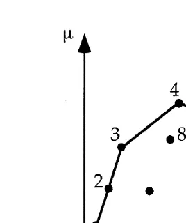
This section provides a pictorial example set in a normal world with a degenerate target. When + is a set of normal distributions and the agent’s ranking is compatible with expected utility as discussed in Section 2.4, we can simplify the representation of the choice set and replace a lottery X by the pair (m, s) of its expected value and standard deviation; see Meyer (1987). For instance, if the target is known for sure and therefore coincides with the reference pointn, Theorem A.1 in Appendix A implies that the agent behaves as if choosing the lottery that maximizes (m 2 n) /s.
Fig. 1. An example of a normal world.
X1|N(m1, s1) to be optimal, there must exist a reference point n such that (m 2 n1 ) /
¯
s 5max (m 2 n) /s 5k. This occurs if and only ifm #x1ks for all (s,m)[#with
1 #
equality holding at (s1, m1); or, equivalently, if and only if there exists an hyperplane through (m , s ) supporting # from above (with respect to the m-axis). Therefore, a
1 1
lottery X|N(m,s) can be optimal if and only if (m,s) lies on the upper boundary of the convex hull of #.
To gain some intuition, consider Fig. 1. Only the lotteries corresponding to the points from 1 to 6 can be optimal. Lottery 2 can be optimal although it is not an extreme point; but when 2 is optimal, the agent is indifferent between Lotteries 1, 2, and 3. Lottery 7 is an extreme point, but it cannot be optimal because either 5 or 6 will be preferred. Lottery 8 cannot be optimal, although its expected value is higher than that of most other lotteries.
Order just the lotteries that can be optimal so that they are increasing in the variance. For instance, we have numbered such lotteries in Fig. 1 from 1 to 6. Then the actual optimal choice is increasing in the reference pointn; that is, the higher isn, the higher is the variance of the optimal choice. In fact, given two reference pointsn . n1 2, let X and1
X be respectively optimal in2 n1 andn2. By Theorem A.1, it must be
m 2 n1 1 m 2 n2 1 m 2 n2 2 m 2 n1 2
]]s $]]s and ]]s $]]s .
1 2 2 1
Adding the two inequalities and rearranging terms, we obtain (n 2 n1 2) /s #1 (n 2 n1 2) / s2, from which s $ s1 2.
normal distributions, see Hanoch and Levy (1969), the agent is risk averse (respectively, risk seeking) when her reference point is sufficiently low (or high).
3.4. Two counterexamples
The main results in this paper are two. First, reference-dependent preferences may converge in the long run. Second, they may lead to risk neutral behavior. This section provides two simple counterexamples, one for each result. Their purpose is to help the reader assess the strengths and the limitations of our approach.
We show first that preferences may fail to converge because the reference point may cycle forever. Recall that we took the reference point to be (essentially) the sample mean of the outcomes received in the past. For simplicity, suppose that the target is degenerate and equal ton. The choice set+ contains two lotteries: X is normally distributed with expected valuem 50 and standard deviations 520; and Y is a (non-symmetric) binary lottery which pays 1 with probability 0.9 and 11 with probability 0.1. The expected value of Y is 2.m. Let n be the current reference point.
We claim that the agent strictly prefers X when n .1 and strictly prefers Y when n #1. Forn #1 andn .11, this is immediate. Forn in (1,11], note that X is normally distributed and therefore
P(X$n).P(X$20)5P(X$m 1 s)512F(1)¯0.1587.0.15P(Y$n). As long asn #1, the agent chooses Y in each period. Since the expected value of Y is 2, persisting in this choice generates payoffs that drive the sample mean up untiln .1; at that point, the agent switches to choosing X. But, in turn, the expected value of X is m 50 and this must eventually bring the sample mean down so that the agent switches back to Y. The reference point cannot converge and thus the agent’s choice keeps going back and forth between X and Y forever, while each cycle stretches (on average) over longer and longer periods.
This first counterexample proves that Theorem 2 is not trivial. Our second counterex-ample shows that, even when the reference point converges, the long run choice behavior may not be risk neutral. This suggests that our model may be used to explain convergence of long-run behavior to different kinds of risk attitudes in worlds which are not symmetric. For the moment, we must leave this conjecture to future research.
Assume again a degenerate target and a choice set with two lotteries: X|N(0, 20) as before and another (non-symmetric) binary lottery Z which pays21 with probability 0.9 and 10 with probability 0.1. Similarly to the above, the agent strictly prefers X when n . 21 and strictly prefers Z whenn # 21. Thus, as far asn # 21, the agent chooses
Z. Since the expected value of Z is 0.1, this must eventually drive the sample mean over 21 and make the agent pick X. Once the agent starts choosing X, which hasm 50, the sample mean tends to settle around 0. Eventually, the reference point converges to 0 and the agent prefers X although Z has a higher expected value. In other words, the agent learns to make a (strictly) risk averse choice.
expected value strictly higher thann, the agent does not content herself with any lottery whose expected value is lower than n. If the agent is ambitious for all values ofn , m* (and if she prefers X* at n 5 m*), then her choice behavior will converge to risk neutrality. In the second counterexample above, ambition fails forn in [0, 0.1) and this prevents convergence to the risk neutral choice.
We note one last important feature of our model. Establishing Theorem 1 suffices to prove Theorem 2 and therefore to obtain convergence to risk neutrality. We proved Theorem 1 using Theorem A.3, which relies on the assumption of a symmetric world. However, there may different ‘worlds’ in which Theorem 1 is true. In any of them, the choice behavior would converge to risk neutrality by Theorem 2. This suggests how to go about proving a piece of our conjecture above: risk neutrality may also emerge in worlds that are not symmetric.
3.5. Changing preferences and expected utility
As the reference point changes, so do the short-run preferences of the agent. It is instructive to consider how their dynamics looks like in both our target-based model and the expected utility model. We begin from the first one.
At the beginning of period t, we can write the target
t t t
¯ V 5x 1z
t t
¯
as the sum of the current reference point x and a random termz . This allows one to model situations where the agent is uncertain about which reference point she should
t
¯
use. For instance, the agent may feel that the average experienced payoff x is an undistorted estimate of the ideal reference point, but that there might be some other relevant (yet unavailable) information that she should take into account. This in-formation combines into a probabilistic assessment of the aspiration level at each period
t.
t
¯
Given that convergence in our model only requires convergence of x , the possible dynamics of these probabilistic assessments includes many possible cases. For instance,
t t
we could assume that the standard deviation s of the target V is decreasing over time as the sample of experienced payoffs becomes longer: the greater the sample, the lower the
t t t
¯
uncertainty. Alternatively, we might assume that s 50 if x ,m* and s .0 otherwise; t
¯
that is, the agent feels confident that x is her target when there is at least one lottery in + that has a higher mean, but entertains doubts once she realizes that her reference point may be too high. More generally, provided that (3) holds, our model is compatible with
t t t
¯
any updating rule for V . We do not even require V to converge, although x will. Hence, in our model based on a random target, the aggregation of short-run preferences into a long-run preferences is compatible with a large class of probabilistic assessments and updating rules. The agent is not required to have a utility function and her preferences change simply because her opinions change.
t t t t11 t substantial. Given V , let U be its corresponding c.d.f. When V is updated to V , U
t11 t
becomes U . The equivalence requires that U be used as utility function in the expected utility representation of the agent’s behavior. Therefore, the same dynamics
t
ensues if we postulate that the utility function U changes its shape over time while the reference point independently evolves so that (3) holds. But it would take a quite
t
contrived story to explain why and how U shifts over time. The model would manage to describe the dynamics of preferences only by ignoring the issue of why they are changing.
4. Conclusions
The adaptive process described in this paper seems close to the learning experience underlying the formation of expertise. Suppose that an inexperienced agent sets her aspiration level too low (or too high). If she exhibits a dual risk attitude, her choices will lead to outcomes that systematically overshoot (or undershoot) the target. As her experience grows, she learns to set more realistic targets and to make choices matching (on average) her aspiration level. Moreover, this process tends to maximize the expected value of the chosen lotteries. Experience is embodied in the evolution of the target and in the stabilization of the reference point at the ‘right’ level.
Unfortunately, we are not aware of any experimental evidence which bears on this interpretation. More generally, the literature lacks attempts to study the evolution of risk attitudes over time. It may be time to undertake such an investigation. Behavioral economics is becoming increasingly aware that preferences are often endogenous and that they may be learnt. However, what (if anything at all) can be eventually learnt is not yet clear.
This paper proposes a model which makes testable predictions about the evolution of choice behavior over symmetric lotteries. In particular, it would be interesting to study the risk attitudes of experienced versus inexperienced agents in a symmetric world. We predict that the first group would be more likely to engage in risk neutral choices.
Acknowledgements
We thank Drew Fudenberg, Bruno Jullien, Mark Machina, Alessandro Rota, two very perceptive referees and seminar audiences at the universities of Alicante, CalTech, London (UCL), San Diego (UCSD), Toulouse and Trento for helpful comments. An earlier version of this paper was written while the second author was visiting the Department of Economics at the University of Toronto. We gratefully acknowledge financial support respectively from Bocconi University and MURST.
Appendix A
Theorem A.1. Suppose that X|N(m,s) and V|N(n, s) are stochastically independent
2 2
m 2 n ]]] P(X$V )5F
S
]]D
2 2
Œ
s 1s2 2
whereF is the distribution function of a standard normal. If insteads 5s 50, then P(X$V )51 ifm $ n and 0 otherwise.
]]2 2
Œ
s
d
Proof. The difference of the two normals V and X is (V2X )|N (n 2 m), s 1s . If
2 2
s 1s .0, we have that
(V2X )2sn 2 md
]]]]] Z5
Œ
]]2 2s 1s
is a standard normal and therefore
m 2 n m 2 n
]]] ]]]
P(X$V )5P(V2X#0)5P Z
S
#Œ
]]2 2D S
5FŒ
]]2 2D
.s 1s s 1s
2 2
If instead s 5s 50, both X and V are degenerate and P(X$V )5P(m $ n). h
Theorem A.2. Given a target V|N(n, s) with s.0 and a lottery X|N(m, s), there
exists a in [0, 1] such that the certainty equivalent CE(X ) satisfies
CE(X )5am 1(12a)n.
Proof. By Theorem A.1, CE(X ) must satisfy
m 2 n CE(X )2n
]]]
Œ
]]2 25]]]s .s 1s
Rearranging, we obtain
m 2 n 1 1
]]]] ]]]] ]]]]
CE(X )5n 1 ]]]5
S
]]]D S
m 1 12 ]]]D
n2 2 2 2 2 2
Œ
11s
s /sd
Œ
11s
s /sd
Œ
11s
s /sd
and the result follows by taking
1 ]]]] a 5
S
Œ
]]]2 2D
. h11
s
s /sd
Theorem A.3. Let X|F and V|U be stochastically independent and symmetrically
distributed, with medians respectivelym andn. Suppose that F is absolutely continuous
and has full support on R. Then
(i ) m 5 n implies P(X$V )51 / 2; (ii ) m . n implies P(X$V ).1 / 2; (iii ) m , n implies P(X$V ),1 / 2.
Proof. Recall that P(X$V )5e U(x) dF(x). Case (i) follows immediately by the
U(x) ifx$m A(x)5
H
U(x22d) ifx,m
Note that A(x) is bounded and symmetric around m. Moreover, U(x)$A(x) for all x.
Therefore,
1 ] P(X$V )5
E
U(x) dF(x)$E
A(x) dF(x)5 ,2
where the last equality follows by the symmetry of A and the absolute continuity of F. To strengthen the inequality, note that there must exist an interval [a, b] in (2`, m) where U(x).A(x). By the full support assumption, F puts positive probability on I and
therefore the strict inequality holds. The proof of Case (iii) follows by reversing the argument just used for Case (ii). h
We say that a random variable V has a unimodal distribution U if there exists a mode ninRsuch that U is convex on (2`,n] and concave on [n, 1 `). If U is unimodal, the set of its modes is a (possibly degenerate) interval. If U is unimodal and has a unique mode n, it may fail to be continuous at (and only at) n; in particular, any degenerate distribution is unimodal.
Theorem A.4. Suppose that the target has a unimodal distribution. Under the
assumptions of Theorem A.3, if there is a certainty equivalent c(X ) for X then there
exists a in [0, 1] such that c(X )5am 1(12a)n.
Proof. Recall that c(X ) solves the equation P(X$V )5P(c$V ). We distinguish three
cases. First, suppose thatm 5 n. By Theorem A.3, P(X$V )51 / 2. Hence, P(c$V )51 / 2 and so c5n. Therefore, c5m 5 n and anya will do. Second, suppose thatm . n. By Theorem A.3, P(X$V ).1 / 2 and so c$n. To prove the result, we need to show that m $c or, equivalently, that
U(c)2U(m)5
E
fU(x)2U(m) dF(x)g #0. Letd 5 m 2 n .0. Define the auxiliary functionU(x)2U(m) if x$m A(x)5
H
U(x22d)2U(m 22d) if x,m
Note that A(x) is bounded and symmetric aroundm, with A(m 1x)1A(m 2x)50 for almost all x. Moreover, A(x)$U(x)2U(m) for all x by the unimodality of U. Therefore, by the symmetry of A,
E
fU(x)2U(m) dF(x)g #E
A(x) dF(x)50,The next theorem is a variation on an almost sure convergence result that is well-known in the literature on stochastic approximation algorithms. Given some
]0
arbitrary random variable X , consider the stochastic algorithm
1
]t11 t t t
¯ ]] ¯
X 5x 1 H(x , X ), (A.1)
t11
where H(x, X ) is a deterministic function. We provide a sufficient condition for the almost sure convergence of (A.1) to a point. Our proof uses an elegant argument developed in Robbins and Siegmund (1971), where the following lemma is proved.
t t t t t
Lemma 3. Leth^ jbe an increasing sequence ofs-algebras. Suppose that Z , A , B , C t
are nonnegative^ -measurable random variables such that
t11 t t t t t
E Z
f
u^g
#Z (11A )1B 2C for all t51, 2, . . . Then, on the set1` 1`
t t
O
A , `,O
B , ` ,H
t51 t51J
t 1` t
it almost surely occurs that Z converges to a finite random variable Z and o C is
t51
finite.
t 0 1 t21
Theorem A.5. Let^ be thes-algebra generated by
h
X , X , . . . , Xj
. Suppose that (A.1) satisfies the following three assumptions:t t t
¯
(i ) the term H(x , X ) is^ -measurable for all t; (ii ) there exists a constant k.0 such that
t 2
2
¯ ¯
E H(x, X )
f
s d u^g
#k 1s
1uxud
¯for all t and all x;
(iii ) for
t t
¯ ¯
h (x )5E H(x, X )
f
u^g
,which is well defined by (ii ), there exists m* such that´ .0 implies t
¯ ¯
sup (x2m*) h (x )#g ¯
´ #ux2m*u#( 1 /´)
]
t t
for someg ,0 which depends on ´ but not on t or on the events in ^ . Then X
converges almost surely to m .
*
t t 2
¯
Proof. Define Z 5(x 2m*) and, for notational simplicity, let at51 /(t11). Then t11 t t t t 2 t t 2
¯ ¯ ¯
Z 5Z 12a (xt 2m*)H(x , X )1at
f
H(x , X )g
. t 2 t 2¯
t11 t t t t t t 2 t t 2 t
¯ ¯ ¯
E[Z u^ ]5Z 12a (x 2m )E[H(x , X )u^ ]1a E[(H((x , X )) u^ ]
t * t
t t t t 2 t 2
¯ ¯ ¯
#Z 12a (xt 2m*)h (x )1ka (1t 1uxu )
t 2 2 2 t t t
¯ ¯
#Z (112ka )t 1ka (1t 12m*)12a (xt 2m*)h (x ).
t 2 t 2 2 t t t t t
¯ ¯
Let A 52ka , Bt 5ka (1t 12m*) and C 5 22a (xt 2m*)h (x ). Note that oA , `,
t t
oB , `and that C is nonnegative by (iii). Therefore, Lemma 3 implies that it almost
t t t t
¯ ¯
surely occurs that Z converges to Z and that oa (xt 2m*)h (x ) is finite.
It remains to show that Z50 almost surely. Proceed by contradiction and suppose t
¯
that Z(v)±0. Then there exist some´ .0 and some T such that´ #ux 2m*u#(1 /´) t t t
¯ ¯
for all t$T. By (iii), supt$T(x 2m*)h (x )#g ,0. But oa diverges and thereforet t t t
¯ ¯
oa (xt 2m*)h (x ) cannot be finite. h
t t t t
¯ ¯
Proof of Theorem 2. Eq. (5) is a special case of (A.1) where H(x , X )5X 2x and
t t
the lottery X 5B(V ) is the optimal choice at time t. Therefore we only need to check
that the three assumptions of Theorem A.5 are satisfied. Assumption (i) holds because
t t
the optimal choice X 5B(V ) is a stochastically independent lottery. Let sM be the greatest standard deviation attainable in the (finite) set +. Then Assumption (ii) holds because
t t 2 t t t 2 t t t 2
¯ ¯
E
f
s
X 2xd
u^g
5Ef
s
B(V )2b(V )d
u^g
1f
b(V )2xg
2 2 t 2
¯ #s 1M 2[m 1* (x ) ].
t t t t
¯ ¯ ¯
Finally, since h (x )5b (V )2x , Assumption (iii) holds because ux2m*u$´ implies t
¯ ¯
(x2m*) h (x )# 2´ ?minh´,hj,0. h
References
Blum, J.R., 1954. Approximation methods which converge with probability one. Annals of Mathematical Statistics 25, 382–386.
Bordley, R.F., LiCalzi, M., 2000. Decision Analysis using Targets instead of Utility Functions. Decisions in Economics and Finance 23, forthcoming.
¨
Borgers, T., Sarin, R., 1996. Naive Reinforcement Learning with Endogenous Aspirations. Mimeo, February. Castagnoli, E., LiCalzi, M., 1996. Expected utility without utility. Theory and Decision 41, 281–301. Dekel, E., Ely, J.C., Yilankaya, O., 1998. Evolution of Preferences. Mimeo, July.
Fishburn, P.C., Kochenberger, G.A., 1979. Two-piece von Neumann–Morgenstern utility functions. Decision Sciences 10, 503–518.
Friedman, M., Savage, J.L., 1948. The utility analysis of choices involving risk. Journal of Political Economy 56, 279–304.
Gigerenzer, G., 1996. On narrow norms and vague heuristics: A reply to Kahneman and Tversky (1996). Psychological Review 103, 592–596.
Gilboa, I., Schmeidler, D., 1996. Case-based optimization. Games and Economic Behavior 15, 1–26. Hanoch, G., Levy, H., 1969. The efficiency analysis of choices involving risk. Review of Economic Studies
36, 335–346.
Heath, C., Huddart, S., Lang, M., 1999. Psychological factors and stock option exercise. Quarterly Journal of Economics 114, 601–627.
Kahneman, D., Tversky, A., 1979. Prospect theory: an analysis of decision under risk. Econometrica 47, 263–291.
LiCalzi, M., 2000. A Language for the Construction of Preferences under Uncertainty. Journal of the Royal Spanish Academy, forthcoming.
Ljung, L., Pflug, G., Walk, H., 1992. Stochastic Approximation and Optimization of Random Systems. ¨
Birkhauser, Boston.
Marimon, R., 1997. Learning from learning in economics. In: Kreps, D.M., Wallis, K.F. (Eds.). Advances in Economics and Econometrics: Theory and Applications, Vol. I. Cambridge University Press, Cambridge, UK, pp. 278–315.
March, J.G., 1996. Learning to be risk averse. Psychological Review 103, 309–319. Markowitz, H., 1952. The utility of wealth. Journal of Political Economy 60, 151–158.
Meyer, J., 1987. Two-moment decision models and expected utility maximization. American Economic Review 77, 421–430.
Robbins, H., Monro, S., 1951. A stochastic approximation method. Annals of Mathematical Statistics 22, 400–407.
Robbins, H., Siegmund, D., 1971. A convergence theorem for non negative almost supermartingales and some applications. In: Rustagi, J.S. (Ed.), Optimizing Methods in Statistics. Academic Press, New York, pp. 233–257.
Robson, A.J., 1996. The evolution of attitudes to risk: lottery tickets and relative wealth. Games and Economic Behavior 14, 190–207.