Full Terms & Conditions of access and use can be found at
http://www.tandfonline.com/action/journalInformation?journalCode=ubes20
Download by: [Universitas Maritim Raja Ali Haji] Date: 11 January 2016, At: 19:31
Journal of Business & Economic Statistics
ISSN: 0735-0015 (Print) 1537-2707 (Online) Journal homepage: http://www.tandfonline.com/loi/ubes20
Evaluating the Calibration of Multi-Step-Ahead
Density Forecasts Using Raw Moments
Malte Knüppel
To cite this article: Malte Knüppel (2015) Evaluating the Calibration of Multi-Step-Ahead
Density Forecasts Using Raw Moments, Journal of Business & Economic Statistics, 33:2, 270-281, DOI: 10.1080/07350015.2014.948175
To link to this article: http://dx.doi.org/10.1080/07350015.2014.948175
View supplementary material
Accepted author version posted online: 31 Jul 2014.
Submit your article to this journal
Article views: 182
View related articles
Evaluating the Calibration of Multi-Step-Ahead
Density Forecasts Using Raw Moments
Malte K
NUPPEL¨
Deutsche Bundesbank,Wilhelm-Epstein-Str. 14, D-60431 Frankfurt am Main, Germany ([email protected])
The evaluation of multi-step-ahead density forecasts is complicated by the serial correlation of the cor-responding probability integral transforms. In the literature, three testing approaches can be found that take this problem into account. However, these approaches rely on data-dependent critical values, ignore important information and, therefore lack power, or suffer from size distortions even asymptotically. This article proposes a new testing approach based on raw moments. It is extremely easy to implement, uses standard critical values, can include all moments regarded as important, and has correct asymptotic size. It is found to have good size and power properties in finite samples if it is based on the (standardized) probability integral transforms.
KEY WORDS: Density forecast evaluation; Moment test; Normality test; Probability integral transfor-mation.
1. INTRODUCTION
Today, predictions are often made in the form of density fore-casts. Tay and Wallis (2000) gave a survey of the use of density forecasts in macroeconomics and finance. Like point forecasts, density forecasts should be evaluated to investigate whether they are specified correctly. Point forecasts, for example, can be tested for bias. Density forecasts, in general, are tested for calibration. Correct calibration means that the density forecast coincides with the true density of the predicted variable.
This work is concerned with the question, how an evaluation of density forecasts can be conducted if the probability integral transforms (henceforth PITs) are serially correlated. The PIT is the probability of observing a value smaller than or equal to the actual outcome according to the forecast density. Serial correlation of the PITs is a typical feature of multi-step-ahead forecasts.
If the density forecasts are calibrated correctly, the PITs are
uniformly distributed over the interval (0,1), as noted by Dawid
(1984), Diebold, Gunther, and Tay (1998), and Diebold, Tay, and Wallis (1999). The original idea for this evaluation approach dates back to Rosenblatt (1952). If the PITs are independent, they can be used directly for testing the calibration of density forecasts, employing, for example, the Kolmogorov–Smirnov test. Applying an inverse normal transformation to the PITs yields, in the case of correctly calibrated density forecasts, a variable with standard normal distribution (henceforth the INTs, i.e., the inverse normal transforms). This second transformation was proposed by Smith (1985) and Berkowitz (2001).
For one-step-ahead forecasts, the PITs (and the INTs), in ad-dition to uniformity (to standard normality), should display in-dependence. In the words of Mitchell and Wallis (2011), if both
conditions are fulfilled, the density forecasts arecompletely
cal-ibrated. The likelihood ratio test proposed by Berkowitz (2001) can be applied to the INTs to test simultaneously for zero mean, unit variance, and zero autocorrelation based on a first-order au-toregressive model (henceforth AR(1)-model) for the INTs. For multi-step-ahead mean forecasts, even optimal forecasts pro-duce serially correlated forecast errors, and the same holds for
completely calibrated density forecasts, which produce serially correlated PITs and INTs. The evaluation of multi-step-ahead forecasts found in the literature, mostly therefore, focuses on correct calibration only. Basically, three approaches can be dis-tinguished.
One approach, proposed by Corradi and Swanson (2006a) and Rossi and Sekhposyan (2014), uses Kolmogorov-type or Cram´er-von-Mises-type tests that account for the serial cor-relation of the data. However, for these tests, critical values are data dependent. Another approach rests on normality tests for the INTs which are valid in the presence of serial correla-tion. Mitchell and Wallis (2011) mentioned the skewness- and kurtosis-based normality tests proposed by Bai and Ng (2005). Corradi and Swanson (2006b) also suggested, inter alia, the tests proposed by Bai and Ng (2005), and related GMM-type tests
introduced by Bontemps and Meddahib (2005,2012). The tests
of Bai and Ng (2005) were employed by D’Agostino, Gambetti, and Giannone (2013) for the evaluation of their density fore-casts. Finally, in several applications like those by Clements (2004), Mitchell and Hall (2005), Jore, Mitchell, and Vahey (2010), Bache et al. (2011), and Aastveit et al. (2011) one finds a variant of the test by Berkowitz (2001) adapted to the case of serially correlated INTs. Instead of testing for zero mean, unit variance and zero autocorrelation, only the first two hypotheses enter the test. Thus, no restriction is placed on the autoregressive coefficient of the AR(1)-model.
Unfortunately, each of the approaches mentioned has cer-tain disadvantages. As stated above, the tests by Corradi and Swanson (2006a) and Rossi and Sekhposyan (2014) rely on data-dependent critical values, which might be a serious imped-iment for their use by practitioners. Concerning the normality tests proposed above, none of them was originally derived to
© 2015American Statistical Association Journal of Business & Economic Statistics
April 2015, Vol. 33, No. 2 DOI:10.1080/07350015.2014.948175
Color versions of one or more of the figures in the article can be found online atwww.tandfonline.com/r/jbes. 270
evaluate density forecasts. Therefore, these tests are based on skewness and kurtosis, but ignore the information contained
in first and second moments. Since the INTs have astandard
normal distribution under the null hypothesis of correct calibra-tion, large power gains could be achieved by considering those moments. Finally, the test by Berkowitz (2001) is based on the assumption of an AR(1)-process. If this assumption is incorrect, the standard critical values are not valid, so that the test does not have the correct asymptotic size. Moreover, for this test, information from higher-order moments is not employed. As in the case of the normality tests, the evaluation of multi-step-ahead forecasts is not the intended use of the test by Berkowitz (2001). Apparently, the tests mentioned have been applied due to the lack of simple tests specifically designed for this task. The raw-moments tests proposed in this work are intended to help close this gap. They do not suffer from any of the disadvantages mentioned, as they use standard critical values, can employ all moments regarded as important, and have correct asymptotic size.
The effects of estimation uncertainty for the parameters of the forecasting model on the evaluation of density forecasts are not addressed in this work. Put differently, the tests presented here are designed for density forecasts which take the parame-ter uncertainty of the underlying model properly into account, or for density forecasts from models with negligible parame-ter uncertainty. Moreover, the results of Rossi and Sekhposyan (2014) imply that density calibration tests, if they are based on the PITs or INTs, are valid for the evaluation of density forecasts at the estimated parameter values of the forecasting model, if the model is estimated under a rolling or fixed scheme. If the densities are to be evaluated at the pseudotrue parameters of the forecasting model, moment-based calibration tests can be modified accordingly as shown in Chen (2011).
The tests proposed in this work can also be used to test for correct calibration of one-step-ahead forecasts. In this case the tests are robust to serial correlation of the PITs, whereas the commonly used tests would suffer from size distortions.
2. CALIBRATION TESTS BASED ON RAW MOMENTS
Let the continuous random variable of interest be denoted
byxt and the forecast density for this variable in period tby
ˆ
f(xt), where the forecast was made in periodt−h,andhis
a positive integer. Many of the methods used for producing density forecasts can be found in the references mentioned in
Section1. The PIT proposed by Rosenblatt (1952) is given by
ut =Fˆ(xt)=
xt
−∞ ˆ
f(q)dq,
where ˆF(xt) denotes the forecast distribution function
associ-ated with ˆf(xt). If the forecast density ˆf(xt) is equal to the true
densityg(xt), thenut is uniformly distributed over the interval
(0,1) (henceforth referred to asU(0,1) distributed). The INT
proposed by Smith (1985) and Berkowitz (2001) is given by
zt=−1(ut)=−1( ˆF(xt)),
where −1(·) is the inverse of the standard normal
distribu-tion funcdistribu-tion. Under the null of correct calibradistribu-tion, zt has a
standard normal distribution. I will proceed under the common
assumption that zt follows a Gaussian process under the null.
However, it should be noted that there are special nonlinear
pro-cesses where the marginal distribution ofzt witht =1,2, . . .
is standard normal, although the joint distribution is nonnor-mal. Tsyplakov (2011) described a strategy for generating such
sequences ofzt.
To test for correct calibration when the PITs are serially cor-related, practitioners have often used a variant of the test pro-posed by Berkowitz (2001), which was apparently first applied by Clements (2004). It is a likelihood-ratio test for the
zero-mean and unit-variance property ofzt, wherezt is assumed to
follow an AR(1)-process. This test will be referred to as the ˆβ12
test. The other existing test that will be employed in this work is
the ˆµ34test by Bai and Ng (2005) which is based on the
skew-ness and kurtosis ofzt, using an estimated long-run covariance
matrix.
The major complications when testing skewness and kurtosis arise from the fact that the expectation and the variance are unknown and, thus, have to be estimated. Therefore, a
four-dimensional covariance matrix is needed for the ˆµ34test, which
is a joint test of only two moments. When testing forstandard
normality, however, also the expectation and the variance are known under the null. Therefore, one does not need to consider standardized moments like skewness and kurtosis. It is not even necessary to employ central moments like the variance. Instead,
nonstandardized, noncentral moments, that is therawmoments
can be employed, so that tests can be constructed very easily. Moreover, raw moments can be estimated unbiasedly in small samples.
Actually, the raw-moments tests do not have to be based on the standard normal distribution, but any suitable transformation of the PITs can be used. Denote the transformed variables by
yt =H(ut),
whereH(ut) is a real-valued function, andH(ut)=−1(ut)
yields standard normally distributed variablesyt =ztunder the
null. Assuming thatE[|yr
ference between both vectors mentioned, is given by
ˆ
long-run variance ofyri
t −mri byσ
fulfilled, as shown by Sun (1965) and Breuer and Major (1983).
Thus, if the latter condition and the conditionE[m2rN]<∞are
fulfilled, every element of √TDˆr
1r2...rN is asymptotically
nor-mally distributed, because E[m2rN]<∞ implies that all
mo-ments of lower order are finite as well (see, e.g., Billingsley 1995, p. 274). From the Cr´amer-Wold device, it then follows
that √TDˆr
1r2...rN converges to a multivariate normal
distribu-tion, that is,
wherer1r2...rN is the long-run covariance matrix of the vector
series
Thus, a test of the distributional assumption forytcan be based
on the statistic
is symmetric around 0, and if at least one odd and one even raw moment are considered, there is an alternative approach that, asymptotically, leads to the same results as the tests described above, but behaves differently in small samples. This approach
is based on the fact that the long-run covariance ofyri
t −mriand yrj
t −mrjequals 0 ifytis symmetrically distributed around 0 and
ifri+rj is odd. A proof of this property is given in Appendix
A. Obviously, since ˆmriand ˆmrjare asymptotically normal, they
are asymptotically independent if they are uncorrelated. Based on this property, one can construct an alternative test
statistic ˆα0
1r2...rN are calculated in the same way as the test
statis-tic ˆαr1r2...rN in (1),but only using the odd and even moments,
r1r2...rNare asymptotically independent.
Concerning the choice of the transformationH(ut), natural
candidates are given by the INTs and (a standardized version of) the PITs. Tests based on the INTs however, are found to suffer from large size distortions in small samples, especially if raw moments of order four or higher are considered. This is because the fourth raw moment, like the sample kurtosis, is strongly positively skewed in small samples. Moreover, sample skewness
and sample kurtosis of normal variables are uncorrelated, but strongly dependent in small samples, and the same holds for the third and the fourth raw moments. For more details see, for example, Doornik and Hansen (2008) and the references therein. Therefore, this work focuses on the standardized PITs (hence-forth S-PITs). They are obtained as
yt =
it is a standard uniformly distributed random variable, that is, a uniformly distributed variable with an expectation of 0 and a variance of 1. Its skewness and kurtosis equal 0 and 1.8,
respectively. The density ofyt is given by
f(yt)=
under the null. Otherwise,f(yt) will differ from this functional
form, but positive values of the density will continue to be
restricted to the interval−√3≤yt ≤
√
3.
3. MONTE CARLO SIMULATION SETUP
3.1 The Densities
To assess the size and power properties of the tests presented, Monte Carlo simulations are used, where it is assumed that the density of the variable
xt ∼N(0,1) (3)
is to be predicted. Thext’s are identically, but not necessarily
independently, distributed. The density forecasts used will be
identical for each period t, so that the PITs will be serially
dependent if thext’s are serially dependent.
For the density forecasts, normal, two-piece-normal,
Stu-dent’stand normal mixture distributions are considered. The
normal distribution is employed to create correctly calibrated density forecasts, or forecasts whose expectation or variance dif-fer from the true values of 0 and 1, respectively. The two-piece normal distribution is employed to construct density forecasts with correct expectation and variance, but with incorrect skew-ness and kurtosis. To construct density forecasts with correct expectation, variance, and skewness, but incorrect kurtosis, the
standardized Student’stdistribution is used. Finally, the normal
mixture distribution is set up such that its first four moments are identical to those of a standard normal distribution while the shapes of both densities differ markedly. In Appendix B, the densities are described in detail.
Assuming normality ofxt and nonnormality of the forecast
densities instead of the opposite (nonnormalxtand normal
fore-cast densities) has the convenient implication that the
uncondi-tional distribution of the data, that is, ofxt,is always normal
and does not depend on the serial correlation. However, the applicability of the tests presented does not rely on any
distri-butional assumption with respect toxt or the forecast density.
Actually, as follows from Wallis (2008), the subsequent simula-tion results would be identical if the simulated INTs were used as realizations, and the forecast density was the standard normal
Table 1. Moments of misspecified forecast densities used in Monte Carlo simulations
µ µ2 s k m1 m2 m3 m4
Normal −0.50 1 0 3 −0.50 1.25 −1.63 4.56
Normal 0 1.50 0 3 0 2.25 0 15.19
Two-piece normal 0 1 0.73 3.41 0 1 0.73 3.41
Student’st 0 1 0 9 0 1 0 9
Normal mixture 0 1 0 3 0 1 0 3
NOTE:µdenotes the expectation,µ2the variance,sthe skewness,kthe kurtosis,mitheith raw moment.
forecast density. To be more precise, the realizations ˜xt would
be generated as
˜
xt =−1(F(xt))
withxt as defined in (3), and withF(·) being the distribution
function of the normal, two-piece-normal, Student’stor normal
mixture distributions mentioned above. The forecast density
would be given by ˆf( ˜xt)=φ( ˜xt), whereφ(·) denotes the
stan-dard normal density. This approach would lead to results which would be identical to those described in what follows.
3.2 The Simulation Environment
An MA(1)-process is used to generate dependent standard
normal variablesxt, so thatxtevolves according to
xt =εt+ρεt−1
withεt∼iidN(0,(1+ρ2)−1) fort =1,2, . . . T. If the
fore-cast density is standard normal, this process leads toyt’s which
correspond to those of two-step-ahead density forecasts which are, in the words of Mitchell and Wallis (2011), completely cal-ibrated. That is, in addition to the fact that the density forecasts
are correctly calibrated,ytis independent fromyt−2,yt−3,. . . .
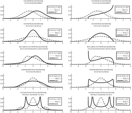
Figure 1. Misspecified forecast densities, the true standard normal densities, and the densities of the corresponding INTs (left column) and S-PITs (right column).
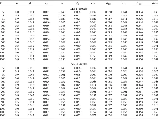
Table 2. Actual sizes of tests
T ρ β12ˆ µ34ˆ α1ˆ αˆ0
12 α12ˆ αˆ
0
123 α123ˆ αˆ
0
1234 α1234ˆ
MA(1)-process
50 0.0 0.051 0.023 0.040 0.036 0.039 0.030 0.041 0.034 0.048 50 0.5 0.035 0.015 0.034 0.033 0.034 0.021 0.023 0.030 0.024 50 0.9 0.024 0.013 0.027 0.029 0.022 0.017 0.011 0.026 0.010 100 0.0 0.051 0.060 0.045 0.043 0.046 0.040 0.048 0.044 0.054 100 0.5 0.034 0.039 0.043 0.044 0.046 0.034 0.043 0.041 0.049 100 0.9 0.024 0.033 0.040 0.040 0.040 0.030 0.035 0.038 0.040 200 0.0 0.050 0.090 0.048 0.046 0.048 0.045 0.049 0.046 0.052 200 0.5 0.032 0.071 0.047 0.048 0.048 0.043 0.048 0.046 0.052 200 0.9 0.023 0.064 0.046 0.047 0.046 0.040 0.045 0.044 0.049 500 0.0 0.050 0.095 0.049 0.048 0.049 0.048 0.050 0.049 0.051 500 0.5 0.032 0.088 0.050 0.050 0.050 0.048 0.050 0.049 0.051 500 0.9 0.024 0.087 0.049 0.050 0.048 0.047 0.048 0.048 0.050 1000 0.0 0.050 0.084 0.049 0.049 0.049 0.049 0.049 0.048 0.050 1000 0.5 0.031 0.085 0.049 0.050 0.050 0.049 0.049 0.049 0.050 1000 0.9 0.023 0.085 0.050 0.051 0.050 0.048 0.049 0.050 0.051
AR(1)-process
50 0.0 0.050 0.023 0.040 0.036 0.039 0.029 0.041 0.034 0.048 50 0.5 0.057 0.012 0.039 0.040 0.046 0.024 0.026 0.034 0.025 50 0.9 0.094 0.002 0.001 0.018 0.000 0.006 0.000 0.004 0.000 100 0.0 0.051 0.059 0.045 0.043 0.046 0.040 0.048 0.043 0.054 100 0.5 0.054 0.029 0.052 0.052 0.063 0.038 0.057 0.047 0.065 100 0.9 0.075 0.002 0.007 0.045 0.014 0.026 0.002 0.044 0.000 200 0.0 0.051 0.091 0.048 0.047 0.048 0.045 0.049 0.047 0.053 200 0.5 0.052 0.057 0.056 0.056 0.061 0.047 0.061 0.051 0.068 200 0.9 0.063 0.006 0.033 0.055 0.053 0.037 0.031 0.073 0.032 500 0.0 0.050 0.095 0.049 0.049 0.050 0.048 0.050 0.049 0.051 500 0.5 0.051 0.083 0.056 0.057 0.058 0.052 0.058 0.053 0.062 500 0.9 0.056 0.018 0.057 0.064 0.081 0.047 0.090 0.068 0.116 1000 0.0 0.051 0.084 0.050 0.050 0.050 0.049 0.050 0.050 0.051 1000 0.5 0.050 0.082 0.055 0.056 0.057 0.054 0.056 0.054 0.058 1000 0.9 0.052 0.041 0.059 0.065 0.073 0.054 0.084 0.065 0.104
NOTE: Actual sizes when the nominal size equals 0.05. Raw-moments tests are based on S-PITs.
Moreover, an AR(1)-process is considered. In this case,xt is
determined by
xt =ρxt−1+εt
withεt∼iidN(0,1−ρ2). The sample sizesT considered are
50, 100, 200, 500, and 1000. The autoregressive and
moving-average parametersρtake on the values 0, 0.5, and 0.9.
The first misspecified normal forecast density considered has
an expectation ofµ= −0.5 and unit variance. The second
mis-specified normal forecast density has an expectation of 0, but
its standard deviation √µ2=σ equals 3/2. The mean-mode
difference γ of the following standardized two-piece normal
forecast density is equal to 0.8. The standardized density of the
t-distribution has 5 degrees of freedom. Finally, the
standard-ized normal mixture density uses the parameter valueσ =0.4.
The moments of these forecast densities are given inTable 1.
The forecast densities, the corresponding densities of the INTs and the S-PITs, and standard normal densities are displayed in Figure 1. In the case of correctly calibrated density forecasts, the density of the S-PITs would be flat and attain a value of
1/√12≈0.3.
The tests considered are the two standard tests employed in the
literature, that is,the ˆβ12test and the ˆµ34test, and various
raw-moments tests based on ˆαr1r2...rNand ˆα
0
r1r2...rN. The parameters for
the ˆβ12test are estimated by maximum likelihood. For the ˆµ34
and the raw-moments tests, the long-run covariance matrices are estimated under the null. That is, the covariances are determined without subtracting the estimated means of the vector series,
which have an expectation of0under the null. With this approach
we follow Bai and Ng (2005). Subtracting the empirical mean would tend to increase the size distortions of the tests, but also improve their power.
Concerning the raw-moments tests, the most parsimonious test is only based on the first moment. Tests with power against more types of density misspecification are obtained by consec-utively adding higher moments. Wherever it is possible, both test statistics, ˆαr1r2...rN and ˆα
0
r1r2...rN,are employed. The largest
moment order considered is 4. This yields the seven test statis-tics ˆα1, ˆα120,αˆ12, ˆα1230 ,αˆ123,αˆ01234,and ˆα1234. As suggested by
Andrews (1991), the quadratic spectral kernel is used for the estimation of the long-run covariance matrix. The truncation lag is also chosen according to Andrews (1991). Employing the Bartlett kernel as in Newey and West (1987) only leads to minor changes of the results.
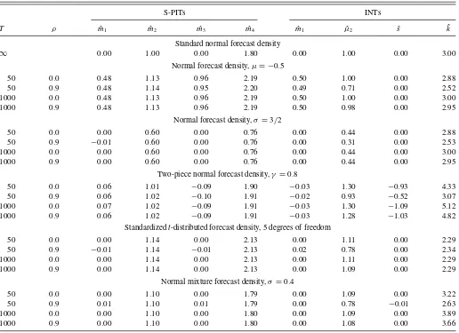
Table 3. Raw sample moments of S-PITs and sample moments of INTs for all forecast densities
S-PITs INTs
T ρ m1ˆ m2ˆ m3ˆ m4ˆ m1ˆ µ2ˆ sˆ kˆ
Standard normal forecast density
∞ 0.00 1.00 0.00 1.80 0.00 1.00 0.00 3.00 Normal forecast density,µ= −0.5
50 0.0 0.48 1.13 0.96 2.19 0.50 1.00 0.00 2.88
50 0.9 0.48 1.14 0.95 2.20 0.49 0.71 0.00 2.52
1000 0.0 0.48 1.13 0.96 2.19 0.50 1.00 0.00 3.00 1000 0.9 0.48 1.13 0.96 2.19 0.50 0.98 0.00 2.95
Normal forecast density,σ=3/2
50 0.0 0.00 0.60 0.00 0.76 0.00 0.44 0.00 2.88
50 0.9 −0.01 0.60 0.00 0.76 0.00 0.31 0.00 2.53 1000 0.0 0.00 0.60 0.00 0.76 0.00 0.44 0.00 3.00 1000 0.9 0.00 0.60 0.00 0.76 0.00 0.44 0.00 2.95
Two-piece normal forecast density,γ =0.8
50 0.0 0.06 1.01 −0.09 1.90 −0.03 1.30 −0.93 4.33 50 0.9 0.06 1.02 −0.10 1.91 −0.02 0.93 −0.52 3.07 1000 0.0 0.07 1.02 −0.09 1.91 −0.03 1.30 −1.09 5.12 1000 0.9 0.06 1.02 −0.09 1.91 −0.03 1.28 −1.03 4.82
Standardizedt-distributed forecast density, 5 degrees of freedom
50 0.0 0.00 1.14 0.00 2.13 0.00 1.11 0.00 2.29
50 0.9 −0.01 1.14 −0.01 2.13 0.02 0.78 0.00 2.34 1000 0.0 0.00 1.14 0.00 2.13 0.00 1.11 0.00 2.29 1000 0.9 0.00 1.14 0.00 2.13 0.00 1.09 0.00 2.29
Normal mixture forecast density,σ =0.4
50 0.0 0.00 1.10 0.00 1.79 0.00 1.09 0.00 3.22
50 0.9 0.01 1.10 0.01 1.79 0.00 0.78 −0.01 2.63 1000 0.0 0.00 1.10 0.00 1.80 0.00 1.09 0.00 3.89 1000 0.9 0.00 1.10 0.00 1.80 0.00 1.08 0.00 3.66
NOTE: ˆmidenotes mean of estimatedith raw moment in 10,000 simulations. ˆµ2,sˆ, and ˆkdenote corresponding values for variance, skewness, and kurtosis, respectively.ρdenotes the
autoregressive coefficient.
To facilitate comparisons between the test statistics, the
size-adjustedpower of the tests will be reported. This requires a
rea-sonably precise estimation of their actual sizes. Using 200,000
Monte Carlo simulations yields an accuracy that appears sat-isfactory for the given purpose, leading to a 95% confidence
interval for the actual size with a width of at most 0.002. The
critical value of the test statistics which is used for the power
computations is determined by the 95% quantile of the 200,000
test statistics computed under the null. For the power
computa-tions, the number of Monte Carlo simulations is set to 10,000,
corresponding to a width of at most about 0.01 for the 95%
confidence interval of the size-adjusted power.
4. SIMULATION RESULTS
4.1 Size
Given a nominal size of 5%, the actual sizes of the ˆβ12test, the
ˆ
µ34 test, and the ˆαr1r2...rN as well as the ˆα
0
r1r2...rN tests based on
the S-PITs are displayed inTable 2. The following statements
concerning the size distortions refer to the absolute differences between the nominal and the actual size, unless otherwise men-tioned.
The size distortions of the raw-moments tests based on the S-PITs are fairly contained. Often, they are considerably smaller if the ˆα0
r1r2...rN tests are used instead of the ˆαr1r2...rN tests. In this
case, the largest negative size distortions are observed for the
case of 50 observations and strong persistence (i.e,in the case
of an AR(1)-process withρ=0.9) with actual sizes often being
below 1%. The largest positive size distortion of the ˆαr01r2...rN
tests is recorded for 200 observations and strong persistence,
where the ˆα12340 test has an actual size of 7.3%. In the case of an
MA(1)-process, the ˆα0r1r2...rN tests always perform well.
If the forecast variable follows an AR(1)-process with no or
only moderate persistence, in general, the ˆβ12 test yields the
smallest size distortions. In the smallest sample and with strong persistence, however, even this test has an actual size of more
than 9%. Given an MA(1)-process, the ˆβ12 test suffers from
size distortions which do not vanish asymptotically. The ˆµ34
test suffers from notable size distortions in many situations. In general, the smallest size distortions of the raw-moments tests
are obtained with the ˆα120 test. While the size distortions of the
ˆ
α1test are often marginally smaller than those of the ˆα012test, in
small samples with strong persistence it underrejects so strongly
that the ˆα012test appears to be preferable. Since, in addition, the
ˆ
α1 test can be expected to have rather low power because it
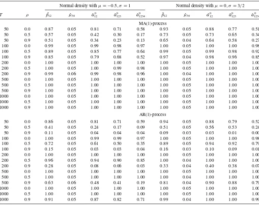
Table 4. Size-adjusted power, normal forecast densities withµ= −0.5,σ=1 and withµ=0,σ =3/2
Normal density withµ= −0.5, σ=1 Normal density withµ=0, σ=3/2
T ρ β12ˆ µ34ˆ αˆ0
12 αˆ
0
123 αˆ
0
1234 β12ˆ µ34ˆ αˆ
0
12 αˆ
0
123 αˆ
0 1234
MA(1)-process
50 0.0 0.87 0.05 0.81 0.71 0.58 0.93 0.05 0.88 0.77 0.51 50 0.5 0.57 0.05 0.42 0.30 0.17 0.73 0.05 0.73 0.65 0.34 50 0.9 0.51 0.05 0.34 0.23 0.13 0.65 0.04 0.64 0.58 0.27 100 0.0 0.99 0.05 0.99 0.98 0.97 1.00 0.05 1.00 1.00 0.98 100 0.5 0.89 0.05 0.85 0.77 0.64 0.99 0.05 0.99 0.98 0.92 100 0.9 0.85 0.05 0.79 0.68 0.52 0.97 0.04 0.98 0.96 0.85 200 0.0 1.00 0.05 1.00 1.00 1.00 1.00 0.05 1.00 1.00 1.00 200 0.5 1.00 0.05 1.00 0.99 0.98 1.00 0.05 1.00 1.00 1.00 200 0.9 0.99 0.06 0.99 0.98 0.96 1.00 0.04 1.00 1.00 1.00 500 0.0 1.00 0.05 1.00 1.00 1.00 1.00 0.05 1.00 1.00 1.00 500 0.5 1.00 0.05 1.00 1.00 1.00 1.00 0.05 1.00 1.00 1.00 500 0.9 1.00 0.05 1.00 1.00 1.00 1.00 0.05 1.00 1.00 1.00 1000 0.0 1.00 0.05 1.00 1.00 1.00 1.00 0.05 1.00 1.00 1.00 1000 0.5 1.00 0.05 1.00 1.00 1.00 1.00 0.05 1.00 1.00 1.00 1000 0.9 1.00 0.05 1.00 1.00 1.00 1.00 0.05 1.00 1.00 1.00
AR(1)-process
50 0.0 0.86 0.05 0.81 0.71 0.59 0.94 0.05 0.88 0.79 0.52 50 0.5 0.41 0.05 0.24 0.17 0.09 0.51 0.05 0.56 0.53 0.24 50 0.9 0.11 0.05 0.04 0.04 0.04 0.09 0.03 0.03 0.01 0.00 100 0.0 1.00 0.05 0.99 0.99 0.97 1.00 0.05 1.00 1.00 0.98 100 0.5 0.72 0.05 0.61 0.50 0.35 0.89 0.05 0.94 0.92 0.79 100 0.9 0.15 0.05 0.03 0.03 0.04 0.16 0.03 0.10 0.09 0.01 200 0.0 1.00 0.05 1.00 1.00 1.00 1.00 0.05 1.00 1.00 1.00 200 0.5 0.96 0.05 0.94 0.90 0.85 1.00 0.04 1.00 1.00 1.00 200 0.9 0.28 0.05 0.08 0.06 0.03 0.33 0.04 0.40 0.38 0.07 500 0.0 1.00 0.05 1.00 1.00 1.00 1.00 0.05 1.00 1.00 1.00 500 0.5 1.00 0.05 1.00 1.00 1.00 1.00 0.04 1.00 1.00 1.00 500 0.9 0.63 0.06 0.48 0.41 0.19 0.81 0.04 0.90 0.88 0.79 1000 0.0 1.00 0.05 1.00 1.00 1.00 1.00 0.05 1.00 1.00 1.00 1000 0.5 1.00 0.05 1.00 1.00 1.00 1.00 0.05 1.00 1.00 1.00 1000 0.9 0.91 0.05 0.87 0.82 0.71 0.99 0.04 1.00 1.00 0.99
NOTE: Raw-moments tests are based on S-PITs.
can only detect misspecifications, which affect the mean of the S-PITs, it will not be considered in what follows.
Summing up, no test can guarantee small size distortions in
all circumstances. However, the ˆα0
r1r2...rN tests based on the
S-PITs always perform well in the case of MA(1)-processes. In the case of AR(1)-processes, they are undersized in small samples
with strong persistence, whereas the ˆβ12test rejects too often in
these cases. The use of the ˆµ34 test and the ˆαr1r2...rNtests cannot
be recommended. Therefore, in what follows, the ˆαr1r2...rN tests
are not considered.
4.2 Size-Adjusted Power
The size-adjusted power (henceforth simply referred to as power) of the tests depends crucially on the sample moments of the S-PITs and INTs. Therefore, these moments are
dis-played in Table 3 for small and large samples (T =50 and
T =1000) and the case of no (ρ=0) and strong (ρ=0.9,
AR(1)-process) persistence. Obviously, the expected sample raw moments do not depend on the sample size or persistence. Differences between the sample raw moments displayed for a
specific forecast density are only caused by the Monte Carlo er-ror. In contrast to the sample raw moments, the sample moment estimators for central and standardized moments can be severely biased.
Turning to the power of the tests, in the case of the
misspec-ified normal forecast densities, the results inTable 4suggest
that, in general, the most powerful test is the ˆβ12 test. It is
su-perior to the other tests especially in small samples with strong
persistence. Otherwise, the ˆα120 test, which is the raw-moment
test corresponding most closely to the ˆβ12test, often has
simi-lar power. The inclusion of higher-order raw moments leads to
power losses. Not surprisingly, the ˆµ34test has power essentially
equal to size.
The misspecifications implied by the two-piece normal fore-cast density are, commonly, most successfully discovered by
the ˆµ34 test and the ˆα0123test, as shown inTable 5. The ˆβ12 test
attains a similar power only ifT =50. The power of the ˆα0
1234
test is comparable to that of the ˆα0
123test. The ˆα012 test has rather
low power, which does not seem surprising, because the mean of the S-PITs is close to 0, and the second raw moment is close
to 1 as shown inTable 3.
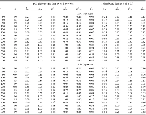
Table 5. Size-adjusted power, two-piece normal forecast density withγ =0.8 and standardizedt-distributed forecast density with 5 degrees of freedom
Two-piece normal density withγ =0.8 t-distributed density with 5 d.f.
T ρ β12ˆ µ34ˆ αˆ0
12 αˆ
0
123 αˆ
0
1234 β12ˆ µ34ˆ αˆ
0
12 αˆ
0
123 αˆ
0 1234
MA(1)-process
50 0.0 0.27 0.24 0.07 0.26 0.23 0.04 0.22 0.13 0.11 0.10 50 0.5 0.25 0.24 0.06 0.19 0.14 0.04 0.17 0.10 0.09 0.08 50 0.9 0.26 0.23 0.06 0.16 0.12 0.04 0.15 0.09 0.10 0.08 100 0.0 0.41 0.59 0.08 0.56 0.52 0.06 0.47 0.23 0.20 0.18 100 0.5 0.37 0.56 0.06 0.45 0.40 0.05 0.39 0.18 0.17 0.16 100 0.9 0.36 0.50 0.07 0.40 0.34 0.05 0.35 0.17 0.15 0.15 200 0.0 0.58 0.94 0.12 0.89 0.88 0.10 0.86 0.48 0.41 0.40 200 0.5 0.55 0.91 0.09 0.82 0.81 0.09 0.80 0.39 0.34 0.34 200 0.9 0.52 0.87 0.08 0.79 0.77 0.08 0.75 0.35 0.30 0.32 500 0.0 0.89 1.00 0.24 1.00 1.00 0.26 1.00 0.89 0.85 0.85 500 0.5 0.84 1.00 0.15 1.00 1.00 0.21 1.00 0.81 0.76 0.79 500 0.9 0.81 1.00 0.14 1.00 1.00 0.20 1.00 0.76 0.70 0.75 1000 0.0 0.99 1.00 0.46 1.00 1.00 0.54 1.00 1.00 0.99 0.99 1000 0.5 0.98 1.00 0.28 1.00 1.00 0.47 1.00 0.99 0.97 0.99 1000 0.9 0.97 1.00 0.24 1.00 1.00 0.42 1.00 0.98 0.96 0.98
AR(1)-process
50 0.0 0.27 0.24 0.07 0.27 0.24 0.04 0.22 0.12 0.11 0.10 50 0.5 0.22 0.24 0.05 0.13 0.10 0.04 0.16 0.08 0.08 0.07 50 0.9 0.14 0.13 0.05 0.06 0.05 0.05 0.06 0.03 0.03 0.06 100 0.0 0.39 0.58 0.09 0.55 0.52 0.06 0.48 0.23 0.20 0.19 100 0.5 0.32 0.54 0.05 0.37 0.31 0.04 0.36 0.14 0.13 0.13 100 0.9 0.17 0.20 0.05 0.07 0.06 0.04 0.08 0.03 0.03 0.05 200 0.0 0.58 0.94 0.12 0.89 0.88 0.09 0.85 0.46 0.40 0.39 200 0.5 0.46 0.88 0.07 0.77 0.75 0.07 0.75 0.31 0.27 0.28 200 0.9 0.22 0.37 0.05 0.11 0.07 0.04 0.13 0.04 0.04 0.05 500 0.0 0.89 1.00 0.24 1.00 1.00 0.25 1.00 0.89 0.84 0.84 500 0.5 0.76 1.00 0.11 1.00 1.00 0.15 1.00 0.72 0.65 0.72 500 0.9 0.30 0.73 0.06 0.43 0.30 0.04 0.44 0.12 0.12 0.16 1000 0.0 0.99 1.00 0.45 1.00 1.00 0.53 1.00 1.00 0.99 0.99 1000 0.5 0.95 1.00 0.18 1.00 1.00 0.34 1.00 0.97 0.94 0.97 1000 0.9 0.45 0.95 0.06 0.87 0.85 0.06 0.84 0.28 0.25 0.42
NOTE: Raw-moments tests are based on S-PITs.
As can also be seen fromTable 5, if the forecast density has
a standardizedt-distribution with 5 degrees of freedom, the ˆµ34
test delivers the best results. Note that this result is related to the fact that the INTs have negative excess kurtosis. For random
variables with positive excess kurtosis, the ˆµ34test has very low
power, as found by Bai and Ng (2005). All raw moments tests attain similar power which here clearly exceeds the power of
the ˆβ12test whenever power exceeds size.
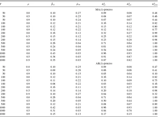
In the case of the normal mixture forecast density, the
behav-ior of the ˆµ34 test reported in Table 6seems counterintuitive
at first sight, because its power appears to decrease with the sample size. However, this can be explained by its asymmetric power properties with respect to excess kurtosis, the bias of the sample kurtosis estimator, and the fact that the sample kurto-sis estimator yields values around 3 in most settings. Broadly speaking, in small persistent samples, the estimated kurtosis is often smaller than 3, and the test has relatively high power in these cases. With even larger sample sizes than considered here,
the power of the ˆµ34test would eventually start to increase. The
ˆ
β12test has relatively low power in almost all cases. The
high-est power, in general, is clearly attained by the ˆα0
1234test. The
high power of the ˆα12340 test compared to all other raw-moments
tests is surprising insofar as, according to Table 3, the fourth
raw sample moment is virtually equal to 1.8, its value under the null. Additional simulations show that, interestingly, the high
power of the ˆα0
1234test stems from the joint consideration of the
second, third, and fourth raw moment. If one of these moments does not enter the test, the power decreases considerably. Ap-parently, the joint distribution of these three sample moments is such that, usually, at least one of the moments is likely to signal departures from the standard uniform distribution.
4.3 Summary
From the Monte Carlo simulations conducted above, it fol-lows that the ˆαr01r2...r
N tests are preferable to the ˆαr1r2...rN tests.
Among the ˆα0r1r2...rN tests, the ˆα120 test tends to give the
small-est size distortions. However, the ˆα12340 test has power against
more types of misspecification, while its size distortions are still
fairly small. Concerning the choice among the ˆβ12test, the ˆµ34
test, and the ˆα0
r1r2...rNtests, the ˆµ34test often has the largest size
Table 6. Size-adjusted power, normal mixture forecast density withσ=0.4
T ρ β12ˆ µ34ˆ αˆ0
12 αˆ
0
123 αˆ
0 1234
MA(1)-process
50 0.0 0.10 0.27 0.09 0.08 0.48
50 0.5 0.10 0.25 0.08 0.07 0.46
50 0.9 0.10 0.24 0.07 0.07 0.44
100 0.0 0.12 0.21 0.16 0.14 0.82
100 0.5 0.12 0.21 0.13 0.12 0.80
100 0.9 0.12 0.22 0.12 0.11 0.77
200 0.0 0.16 0.12 0.32 0.27 0.99
200 0.5 0.15 0.12 0.25 0.22 0.99
200 0.9 0.15 0.14 0.23 0.20 0.98
500 0.0 0.26 0.04 0.71 0.64 1.00
500 0.5 0.24 0.04 0.61 0.55 1.00
500 0.9 0.24 0.05 0.54 0.48 1.00
1000 0.0 0.43 0.03 0.96 0.93 1.00
1000 0.5 0.38 0.03 0.91 0.87 1.00
1000 0.9 0.35 0.03 0.87 0.82 1.00
AR(1)-process
50 0.0 0.10 0.25 0.09 0.08 0.47
50 0.5 0.09 0.26 0.06 0.06 0.41
50 0.9 0.10 0.15 0.05 0.04 0.10
100 0.0 0.12 0.21 0.16 0.14 0.82
100 0.5 0.11 0.22 0.10 0.09 0.75
100 0.9 0.08 0.22 0.03 0.03 0.16
200 0.0 0.16 0.11 0.32 0.27 0.99
200 0.5 0.14 0.14 0.20 0.18 0.98
200 0.9 0.10 0.27 0.04 0.03 0.32
500 0.0 0.26 0.04 0.71 0.64 1.00
500 0.5 0.20 0.05 0.50 0.44 1.00
500 0.9 0.12 0.21 0.08 0.07 0.89
1000 0.0 0.42 0.03 0.96 0.93 1.00
1000 0.5 0.31 0.03 0.84 0.78 1.00
1000 0.9 0.15 0.13 0.17 0.15 1.00
NOTE: Raw-moments tests are based on S-PITs.
distortions, it cannot detect misspecifications which affect first and second moments of the INTs only, and its power can depend in complex ways on sample size and persistence. Therefore, this test does not appear to be well-suited for the evaluation of
density forecasts. The ˆβ12 test has good size properties if the
underlying AR(1)-process assumption is correct, but otherwise suffers from size distortions which do not vanish asymptotically. It appears to be the best choice if the sample size is small, and the data is very persistent. If persistence is only moderate, as
one would expect in the case ofhbeing not too large, or if the
sample is not too small, the ˆα0
1234 test has satisfactory power
against many types of misspecification. Therefore, in general,
the ˆα01234 appears to be the most recommendable test for the
calibration of multi-step-ahead density forecasts.
5. EMPIRICAL APPLICATION
In what follows, the calibration of density forecasts for the logarithm of the daily euro/pound sterling (henceforth EUR/GBP) exchange rate is investigated. The data cover the period from January 4, 2008, to February 28, 2014, and are
displayed inFigure 2. I considerh-step-ahead forecasts withh
equal to 2 and to 3 days.
Denoting the log of the exchange rate at timetby byxt, I
assume thatxt follows a random walk, and that the changes in
xtcan be described by a conditionally heteroscedastic Gaussian
Figure 2. 100 times the logarithm of the daily EUR/GBP exchange rate.
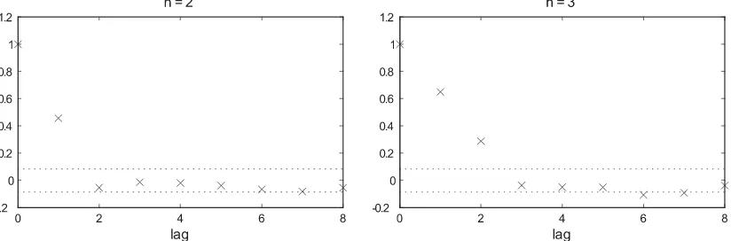
Figure 3. Autocorrelations of the INTs of the density forecasts for the daily EUR/GBP exchange rate for forecast horizonsh=2 andh=3. Dashed lines indicate 95% confidence bounds, calculated as±2/√T.
Table 7. Moments of S-PITs and INTs and test results for calibration of density forecasts for the daily EUR/GBP exchange rate
Moments
S-PITs INTs p-values
ˆ
m1 m2ˆ m3ˆ m4ˆ m1ˆ µ2ˆ αˆ0
1234 αˆ
0
12 β12ˆ
h=2 0.01 0.87 0.02 1.50 0.00 0.85 0.01∗∗ 0.00∗∗∗ 0.12 h=3 0.01 0.86 0.00 1.41 0.00 0.81 0.04∗∗ 0.02∗∗ 0.11
NOTE: Raw-moments tests are based on S-PITs. Sample sizes equalT=555.mˆidenotes theith raw moment, ˆµ2the variance.∗∗∗,∗∗,∗denote rejection at the 1%,5%,10% significance
level.
time series model as in Bollerslev (1986) given by
xt =xt−1+qt, qt=σtεt σt2=b0+b1qt2−1+b2σt2−1
withεt ∼iidN(0,1). A rolling estimation window with 1000
observations is used, andT =555 density forecasts forxt are
evaluated.
The autocorrelations of the resulting INTs are displayed in Figure 3. Obviously, the dynamics of the INTs associated with
the h-step-ahead density forecasts seem to be fairly well
de-scribed by MA(h−1 )-processes. The autocorrelations of the
PITs are very similar to those of the INTs, so that the same statement applies.
To check for correct calibration, the ˆα0
1234 test, the ˆα
0
12 test,
and the ˆβ12test are employed. InTable 7, in addition to the test
results, the first four sample raw moments of the S-PITs as well as the sample mean and variance of the INTs are shown.
The ˆα12340 test rejects the null hypothesis of correct calibration
for both forecast horizons at the 5% significance level. At the
latter level, the ˆα120 test also rejects forh=3, and forh=2 it
rejects at the 1% level. In contrast to that, no rejections occur
with the ˆβ12test. When looking at the moments, it appears likely
that the major misspecification of the forecast densities is their
excessive dispersion. In such a situation, according toTable 4,
the ˆα0
12 test and the ˆβ12 test have similar size-adjusted power.
Yet, the ˆβ12 test is undersized in the presence of an
MA(1)-process with positive MA coefficient, and this property could also hold for MA(2)-processes. This could be a reason why the
ˆ
β12test does not reject here.
6. CONCLUSION
Raw-moments tests for the calibration of multi-step-ahead density forecasts are proposed and compared to two commonly
used tests, the ˆβ12test of Berkowitz (2001), and the ˆµ34 test of
Bai and Ng (2005). These tests employ the inverse normal trans-forms (INTs) of the probability integral transtrans-forms (PITs). The raw-moments tests are based on the standardized PITs (S-PITs). Despite of the autocorrelation of the PITs, the raw-moments tests rely on standard critical values.
It turns out that the ˆµ34 test cannot be recommended for
the evaluation of density forecasts due to potentially large size distortions, complicated power properties, and ignoring
infor-mation from lower-order moments. The ˆβ12 test can be very
useful because of its relatively large power especially in small samples with strong persistence. Yet, if the INTs do not fol-low an AR(1)-process, size distortions occur which do not van-ish asymptotically. Moreover, the test does not use information from higher-order moments.
Tests based on the S-PITs do not suffer from these short-comings, and can therefore, and because of their simplicity, be a very helpful tool for the evaluation of density forecasts. The tests which use the fact that under the null, odd and even sample moments are uncorrelated, perform better in terms of size and power than their counterparts which do not employ
the zero-correlation property. Among the former tests, the ˆα12340
test, which uses the first four raw moments of the S-PITs, has good size and power properties in most settings investigated in this study. Therefore, in general, it appears to be the most recommendable test.
APPENDIX A: PROOF
The following proof shows that the long-run covariance ofyri t −mri andytrj −mrj equals 0 ifyt is symmetrically distributed around 0 and ifri+rjis odd. Consider the standard normal variablezt, and denote the symmetry-preserving transformation byyt =S(zt) whereS(zt) is an odd function. The symmetric density ofytwill be denoted byf(yt). Suppose thatriis odd andrjis even. Then, for the contemporaneous covariance ofyri
t andy
rjdenotes the expectationE[y rj function, implying thatyr
tf(yt) is an odd function. Thus,E[y
For the noncontemporaneous covariance ofyri t andy
Starting withzt, the latter expectation can be rewritten as
E first and the fourth term and the sum of the second and the third term the right-hand side are both equal to 0, so that the entire expression equals 0.
Consideringyri t andy
rj
t instead of the odd functionz ri
t and the even functionzrj
t leads to the same result, because, first,y ri
t also is an odd function andyrj
t also is an even function, and second,f(yt, yt−v)= f(−yt,−yt−v) andf(yt,−yt−v)=f(−yt, yt−v) must hold because yt =S(zt) is a symmetry-preserving transformation. Therefore,
E
Here the densities used for the Monte Carlo simulations are described. Unless otherwise mentioned, their skewness equals 0 and their kurtosis equals 3.
Denoting the standard normal density byφ(·), the normal forecast density is
whereµis the mean andσ the standard deviation ofxt.
The two-piece normal distribution, as described, for example, in Wallis (2004, p. 66), is defined by
withmbeing the mode and with the moments
E[xt]=µ=m+ The parameterγrepresents the mean-mode difference. A positive value ofγcorresponds to a positively-skewed random variablext. Skewness and kurtosis of the standardized two-piece normal distribution are given by
Letτ(xt, v) denote the density function of thet-distribution withv
degrees of freedom withv >4. To obtain a forecast density with unit variance, the scaled forecast density given by
ˆ
is employed. The kurtosis ofxt equals
k= 3v−6 v−4.
Finally, the normal mixture density considered is given by
ˆ
The author thanks J¨org Breitung, Matei Demetrescu, James Mitchell, Barbara Rossi, Karl-Heinz T¨odter, Alexan-der Tsyplakov, Ken Wallis, and participants at the workshop “Uncertainty and Forecasting in Macroeconomics” in Eltville, organized by the Deutsche Bundesbank and the ifo Institute, as well as participants at “The 32nd Annual International Sym-posium on Forecasting” in Boston for helpful comments and suggestions. This article represents the author’s personal opin-ion and does not necessarily reflect the views of the Deutsche Bundesbank.
[Received August 2013. Revised May 2014.]
REFERENCES
Aastveit, K. A., Gerdrup, K. R., Jore, A. S., and Thorsrud, L. A. (2011), “Now-casting GDP in Real-Time: A Density Combination Approach,” Working Paper 2011/11, Norges Bank. [270]
Andrews, D. W. K. (1991), “Heteroskedasticity and Autocorrelation Consistent Covariance Matrix Estimation,”Econometrica, 59, 817–858. [274] Bache, I. W., Jore, A. S., Mitchell, J., and Vahey, S. P. (2011), “Combining
VAR and DSGE Forecast Densities,”Journal of Economic Dynamics and Control, 35, 1659–1670. [270]
Bai, J., and Ng, S. (2005), “Tests of Skewness, Kurtosis, and Normality for Time Series Data,”Journal of Business and Economic Statistics, 23, 49–60. [270,271,274,277,279]
Berkowitz, J. (2001), “Testing Density Forecasts, With Applications to Risk Management,”Journal of Business and Economic Statistics, 19, 465–474. [270,271,279]
Billingsley, P. (1995),Probability and Measure(3rd ed.),New York: Wiley. [272]
Bollerslev, T. (1986), “Generalized Autoregressive Conditional Heteroskedas-ticity,”Journal of Econometrics, 31, 307–327. [279]
Bontemps, C., and Meddahi, N. (2012), “Testing Distributional Assumptions: A GMM Aproach,”Journal of Applied Econometrics, 27, 978–1012. [270] ——— (2005), “Testing Normality: A GMM Approach,”Journal of
Economet-rics, 124, 149–186. [270]
Breuer, P., and Major, P. (1983), “Central Limit Theorems for Non-Linear Functionals of Gaussian Fields,”Journal of Multivariate Analysis, 13, 425– 441. [272]
Chen, Y.-T. (2011), “Moment Tests for Density Forecast Evaluation in the Presence of Parameter Estimation Uncertainty,”Journal of Forecasting, 30, 409–450. [271]
Clements, M. P. (2004), “Evaluating the Bank of England Density Forecasts of Inflation,”The Economic Journal, 114, 844–866. [270,271]
Corradi, V., and Swanson, N. R. (2006a), “Bootstrap Conditional Distribution Tests in the Presence of Dynamic Misspecification,”Journal of Economet-rics, 133, 779–806. [270]
——— (2006b), “Predictive Density Evaluation,” inHandbook of Economic Forecasting(vol. 1), eds. G. Elliott, C. W. J. Granger, and A. Timmermann, North Holland: Elsevier, chapter 5, pp. 197–284. [270]
D’Agostino, A., Gambetti, L., and Giannone, D. (2013), “Macroeconomic Fore-casting and Structural Change,”Journal of Applied Econometrics, 28, 82– 101. [270]
Dawid, A. P. (1984), “Statistical Theory: The Prequential Approach,”Journal of the Royal Statistical Society,Series A, 147, 278–292. [270]
Diebold, F. X., Gunther, T. A., and Tay, A. S. (1998), “Evalu-ating Density Forecasts With Applications to Financial Risk
Management,” International Economic Review, 39, 863–883. [270]
Diebold, F. X., Tay, A. S., and Wallis, K. F. (1999), “Evaluating Density Fore-casts of Inflation: The Survey of Professional Forecasters,” inCointegration, Causality, and Forecasting: Festschrift in Honour of Clive W. J. Granger, eds. R. F. Engle and H. White, Oxford, UK: Oxford University Press, pp. 76–90. [270]
Doornik, J. A., and Hansen, H. (2008), “An Omnibus Test for Univariate and Multivariate Normality,”Oxford Bulletin of Economics and Statistics, 70, 927–939. [272]
Jore, A. S., Mitchell, J., and Vahey, S. P. (2010), “Combining Forecast Densities From VARs With Uncertain Instabilities,”Journal of Applied Econometrics, 25, 621–634. [270]
Mitchell, J., and Hall, S. G. (2005), “Evaluating, Comparing and Combining Density Forecasts Using the KLIC With an Application to the Bank of England and NIESR Fan Charts of Inflation,”Oxford Bulletin of Economics and Statistics, 67, 995–1033. [270]
Mitchell, J., and Wallis, K. F. (2011), “Evaluating Density Forecasts: Fore-cast Combinations, Model Mixtures, Calibration and Sharpness,”Journal of Applied Econometrics, 26, 1023–1040. [270,273]
Newey, W. K., and West, K. D. (1987), “A Simple, Positive Semi-Definite, Het-eroskedasticity and Autocorrelation Consistent Covariance Matrix,” Econo-metrica, 55, 703–708. [274]
Rosenblatt, M. (1952), “Remarks on a Multivariate Transformation,”Annals of Mathematical Statistics, 23, 470–472. [270,271]
Rossi, B., and Sekhposyan, T. (2014), “Alternative Tests for Correct Specifi-cation of Conditional Predictive Densities,” Mimeo, Barcelona Graduate School of Economics, Universitat Pompeu Fabra. [270,271]
Smith, J. Q. (1985), “Diagnostic Checks of Non-Standard Time Series Models,” Journal of Forecasting, 4, 283–291. [270,271]
Sun, T.-C. (1965), “Some Further Results of Central Limit Theorems for Non-Linear Functions of a Normal Stationary Process,”Journal of Mathematics and Mechanics, 14, 71–85. [272]
Tay, A. S., and Wallis, K. F. (2000), “Density Forecasting: A Survey,”Journal of Forecasting, 19, 235–254. [270]
Tsyplakov, A. (2011),Evaluating Density Forecasts: A Comment, MPRA Paper 31184, Germany: University Library of Munich. [271]
Wallis, K. F. (2004), “An Assessment of Bank of England and National Institute Inflation Forecast Uncertainties,”National Institute Economic Review, 189, 64–71. [280]
——— (2008), “Forecast Uncertainty, Its Representation and Evaluation,” in Econometric Forecasting and High-Frequency Data Analysis(vol. 13), eds. R. S. Mariano and Y.-K. Tse, Singapore: World Scientific Publishing Com-pany. [272]