Staff Site Universitas Negeri Yogyakarta

(1)

102906-7575 IJBAS-IJENS © December 2010 IJENS

Study on the Magnetic Field Dependence of the

Nematic-Isotropic Phase Transition of Liquid Crystals

: A Monte Carlo Study by Employing the

Wang-Warner Simple Cubic Lattice Model

Warsono

a

, Kamsul Abraha

b

, Yusril Yusuf

b

, Pekik Nurwantoro

b

a _{Department of Physics Education, Faculty of Mathematics and Natural Science, Yogyakarta State University, 55281 Yogyakarta,} Indonesia

b _{Department of Physics, Faculty of Mathematics and Natural Science, Gadjah Mada University, 55281 Yogyakarta, Indonesia}

Abstract-- We have used Monte Carlo technique by employing the Wang-Warner simple cubic lattice model to study the influence of magnetic field on nematic-isotropic phase transition of liquid crystals. This is shown in phase diagrams involving energy per site, orientational order parameter and specific heat as function of temperature. We find that in the absence of magnetic field, the nematic-isotropic phase transition is a strong first order transition. Upon increasing the strength of magnetic field, the jump of first order phase transition becomes small and

in a critical magnetic field (

h

_c



0

,

3

), the phase transition

changes becoming the second order. For fields larger than

h

_c

there is no phase transition and the nematic and paranematic phases are indistinguishable.

Index Term-- phase transition, liquid crystal, magnetic field, Monte Carlo technique, Wange-Warner simple cubic lattice

1. INTRODUCTION

According to common wisdom, there are three basic states of matter, solid, liquid, and gaseous states. However, this is not generally true. Now, there exist other new states of matter in nature, such as the liquid crystal state, plasma state, amorphous solid, superconductor, neutron state, etc. [1, 2]. Liquid crystals are wonderful materials that they exhibit intermediate state between liquid and solid (crystal). They possess some typical properties of liquid as well as solid states. Crystalline materials or solids are materials characterized by strong positional order and orientational order. The positional and orientational orders have low values for liquids. The liquid crystal phase is a mesophase, which occurs in the transition from solid to liquid (isotropic). As a result, positional order and orientational order of liquid crystals have values between solids and liquids [3, 4]. There are three distinct types of liquid crystals accordance with physical parameters controlling the existence of the liquid crystalline phases: thermotropic, lyotropic and polymeric. The most widely used liquid crystals, and extensively studied are thermotropic liquid crystals [5]. Their liquid crystalline phases controlled by temperature. The three main classes of thermotropic liquid crystals are: nematic, smectic and cholesteric. The nematic phase is the simplest of liquid crystal

phase. In this phase the molecules maintain a preferred orientational direction as they diffuse throughout the sample. There exists orientational order, but no positional order [6]. The orientation of nematic liquid crystals can be controlled by an external fields, particularly electric or magnetic fields [7]. If an external field is applied on the nematic liquid crystals, then the evolution of order parameter can be occurred [8]. So, it is important to understand how is the effect of magnetic field on phase transition of nematic liquid crystals.

In recent years rapid advances in the speed of computers has led to the increased use of molecular simulation as a tool to understand complex systems. In the complex systems, such as liquid crystals, simulation is often difficult, with subtle changes in intermolecular forces leading to changes in phase behaviour. Moreover, in the case of liquid crystals many properties of interest arise from specific ordering of molecules (or parts of molecules) in the bulk; and so can only be studied by simulation of many molecules. Despite these difficulties the progress in molecular simulation has been rapid [9]. In computer simulation, a very popular method to solve the complex system under equilibrium states is Monte Carlo method. This method is applicable for complex systems with characteristics: large number of components, many interactions, large parameter space, uncertainty in value of parameters, and uncertainty in outcomes, while deterministic method is failed.

(2)

lattice has three possibilities values, i.e. spin up (+1), spin down (-1) and spin horizontal or perpendicular (0). The nearest neighboring spin has six orientation possibilities in three-dimensional space. The six orientation possibilities are: one spin is up (+1), one spin is down (-1) and four spins are perpendicular (0) [1].

In this paper, we want to understand the effect of magnetic field on nematic-isotropic phase transition of liquid crystal. We use Metropolis Monte Carlo technique and Wang-Warner simple cubic lattice model to calculate and plot phase diagrams of energy per site, orientational order parameter, and specific heat as function of temperature in various magnetic fields. From the plots, we can unambiguously determine the change of phase transition.

2. WANGE-WARNER CUBIC LATTICE MODEL OF

LIQUID CRYSTAL

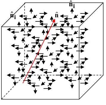
In this model, we consider L x L x L cubic lattice with each lattice sites indexed by number i. Each lattice site holds a molecule director or local director (spin) denoted by a unit

vector

n

ˆ

_i. The average of all local directors that indicates a liquid crystal alignment, usually called director, is denoted by a unit vector

n

ˆ

(see Fig. 1). Each a unit vector

n

ˆ

_i has three possibilities values: 1 for spin-up, -1 for spin-down and 0 for spin-horizontal. The degree of liquid crystal alignment for a set of vector spins,

n

ˆ

_i, is measured via an order parameter [8, 9]:

n)

n

(

_i

2





P

ˆ

S

where

P

₂

(x)



1₂



3

x

2



1



is the second Legendre

polynomial and

...

is an average all the spins .

In the 3D cubic lattice model, each spin in site lattice has six nearest neighboring spins denoted by a unit vector

n

ˆ

_j. Figure 2 shows the six possibilities of spin directions , i.e.

1



j

n

ˆ

,

n

ˆ

_j_₂,

n

ˆ

_j_₃,

n

ˆ

_j_₄,

n

ˆ

_j_₅, and

n

ˆ

_j_₆. The value of

1



j

n

ˆ

is 1,

n

ˆ

_j_₂ is -1,

n

ˆ

_j_₃,

n

ˆ

_j_₄,

n

ˆ

_j_₅ and

n

ˆ

_j_₆ is 0.

The energy of interaction between spin on site and their nearest neighboring spins is modeled by Lebwohl-Lasher [7, 8, 11]:

(2)

)

n

(

_i _j

2









ij

n

J

P

ˆ

E

where

J



0

is the strength of interaction and

ij

indicates nearest neighbors only.

As liquid crystals are anisotropic diamagnetisms, they align in magnetic field. The energy of interaction between spin clusters

n

ˆ

_i (molecular director of liquid crystals) and magnetic field is modeled by [5, 14]:

)

(

)

n

(

)

H

n

(

_i _i _m

3

1 2 2 1 2 2

1

ˆ

h

ˆ

E

N i N i a

m



 

















where



_a





_||





_is a positive diamagnetic anisotropy,

2 2 1 2

H

h





_a , and

n

ˆ

_m is a unit vector parallel to

H



. From Equation (2) and (3), the total energy of the systems (liquid crystals under magnetic field) is:

)

n

(

)

n

(

_i _j _i _m

1 2 2 2







_







N i ij

ˆ

h

ˆ

P

J

E

From thermodynamics, we know that the specific heat is related to the energy of the systems by:

dT

E

d

C

_V



According to the fluctuation-dissipation theorem of statistical mechanics, the variance of the energy is related to the specific heat by [15, 16]:

n

ˆ

i

n

ˆ

[image:2.612.317.567.217.472.2]

i

n

ˆ

Fig. 1. Schematic representation of the local director

n

ˆ

_i

and the director

n

ˆ

of liquid crystal in the Wange-Warner model i

n

ˆ

1  j

n

ˆ

2  j

n

ˆ

3  j

n

ˆ

4  j

n

ˆ

5  j

n

ˆ

6  j

n

ˆ

[image:2.612.120.298.296.472.2]

(3)

 

(6)

T

k

E

C

B

V ₂

2





where

 



E

2



E

2



E

2.

3. MONTE CARLO SIMULATION

The Monte Carlo method is a technique for analyzing phenomena by means of computer algorithms that employ, in an essential way, the generation of random numbers [17, 18]. The term ”Monte Carlo” was given its name by Stanislaw Ulam and John von Neumann, who invented the method to solve neutron diffusion problems at Los Alamos in the mid 1940s. It was suggested by gambling casinos at the city of Monte Carlo in Monaco.

In our Monte Carlo simulation, we used Metropolis algorithm to compute the energy per site, order parameter and specific heat as function of temperature in the magnetic field variations. The procedure of the simulation is described as follow.

a. Determine the parameter constants :

1) The number of lattice size :

N



40

x

40

x

40

2) The strength of interaction :

J



1

3) The Boltzmann’s constant :

k

_B



1

4) The lowest temperature

Ta



0.

01

, the highest

temperature

Tb



1.

11

, the number steps of

temperature

NT



200

, and compute the step of temperature

NT

/

)

Ta

Tb

(

dT





5) The lowest magnetic field

ha



0

, the highest magnetic field

hb



0.

8

, and the steps of magnetic field

1

0.

dh



b. For

h



ha

to

h



hb

with the step

dh

, do : 1) for

T



Ta

to

T



Tb

with step

dT

, do :

a) determine the initial configuration of spins

b) determine the tolerance of spins flip process

1

0.

tol



,

c) determine the number of Monte Carlo loop

4000



NC

and NCA = 3000

d) for the Monte Carlo loops, do :

 calculate the six nearest-neighbors spins of

each spin in a site of lattice

 calculate the change in energy of flipping a

spin



E

 calculate the transition propbabilities:







,

exp

E

/

k

T



min

p



1





_B

 decide which transitions will occur by:

1

+

-2

*

tol

<

N

N,

rand

.*

p

<

N

N,

rand

trans



(

)

(

)

 determine the new configuration of spins

 calculate the variable of interest

E

,

S

, and

V

C

e) calculate the average of

E

,

S

, and

C

_V for 1000 data (from 3000 to 4000 steps)

c. display the diagrams of:

E

vs

T

,

S

vs

T

, and

T

vs

C

_V .

All calculations in this simulation were done using a MATLAB program. These runs took 120.53 hours for

40

x

lattices (or 64.000 molecules), 9 steps of h, 200 steps of T, and 4000 steps of Monte Carlo loops.

4. RESULT AND DISCUSSION

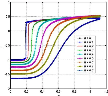
Figure 1 shows energy

E

as a function of temperature

T

, for various values of magnetic field

0.7

0.6,

0.5,

0.4,

0.3,

0.2,

0.1,

0,



h

, and 0.8. For h = 0

(absence of magnetic field), the energy jumps drastically at the critical temperature. The apparent discontinuity of the energy

E suggests that the system has undergone a first order phase transition. For higher h, the jump of first order phase transition becomes small and in the critical magnetic field

3

0

.

h



_c



the jump is disappeared and the second order phase transition is occurred. For h  hc, the energy E becomes

continuous for all the values of magnetic fields. In the figure, it is shown that the temperature transition is higher for larger of magnetic field.

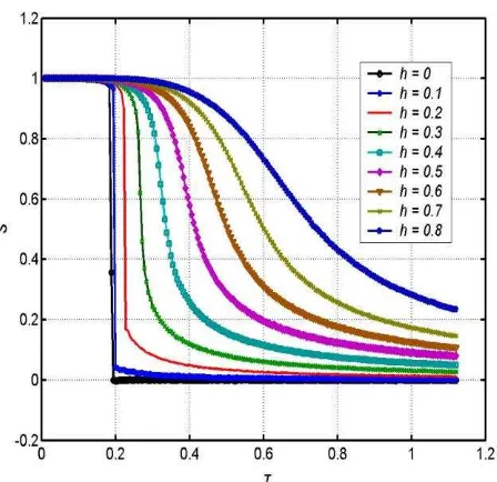
[image:3.612.316.543.353.554.2]

(4)

function of temperature for various values of h. As the same of energy in Figure 1, for the absence of magnetic field (h = 0), the order parameter S jumps drastically at the critical temperature and it clears that the phase transition is first order. Upon increasing the strength of magnetic field (

0



h



h

_c), the jump of the order parameter becomes small and in a critical magnetic field (

h

c



0

,

3

), the order parameter

becomes continuous and the phase transition changes becoming the second order. In the Figure 2, it can be seen that the existence of magnetic field influences to the value of order parameter. In the range of 0 < h < hc and T > Tt, where Tt is

transition temperature, the value of order parameter is higher than zero. It means that the magnetic field induces orientational order in the isotropic phase to the paranematic phase In this region, the nematic phase and paranematic phase are distinguishable. The phase transition is a first order phase transition between nematic and paranematic phase, see [6, 8]. For the magnetic field larger than hc there is no phase

transition and the nematic and paranematic phase are indistinguishable.

Figure 3 describes specific heat CV as a function of

temperature T for various values of h. For h = 0, we find that the specific heat shows a sharp maximum at the transition temperature. Upon the increasing the strength of magnetic field, the sharpness becomes small and in the critical magnetic field hc the sharpness is lost and the second order phase

transition is appeared. This is in agreement Giordano [15].

Figure 4 shows the variation of energy with magnetic field for different values of temperature. In general, for all temperatures, the energy of the system decreases with increases of the magnetic field. For T < Tf (

T

_f



0.

2

is [image:4.612.59.283.72.289.2]

transition temperature in absence of magnetic field, first order transition) and

T



T

_s (

T

_s



0

.

3

is transition temperature of the second order phase transition in existence of magnetic field), the energy is continuous, and in the range

Fig. 2. Orientational order parameter S as a function of temperature T for various values of the magnetic field h.

Fig. 3. Specific heat CV as a function of temperature T for various values of the

magnetic field h.

[image:4.612.330.572.78.279.2] [image:4.612.338.580.413.620.2]

(5)

f

T





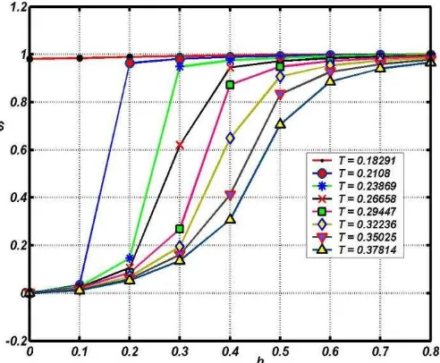
the energy is discontinuous. The discontinuity of E indicates that the phase transition is a first order.

Figure 5 describes the order parameter S as a function of magnetic field h for various values of temperature T. This relation is opposite with the energy versus the magnetic field. The order parameter is increase proportional to the increasing of the magnetic field for all temperatures. A discontinuous jump in S as a function of magnetic field h is found at all temperatures below

T

_s and above

T

_f. In the range of temperature

T

_f



T



T

_s, the order parameter is a discontinuous and it is a first order phase transition. The discontinuity of the order parameter S is similar to the magnetization M of spins on the ising model, see [15]

5. CONCLUSIONS

We have used a Wange-Warner simple cubic lattice model to study the influence of magnetic field on nematic-isotropic phase transition of liquid crystals. The applied of magnetic field on liquid crystal changes the first order phase transition become to the second order and induces the isotropic phase become to the paranematic phase. This is shown in phase diagrams involving energy per site, orientational order parameter and specific heat as function of temperature for the various values of magnetic field.

REFERENCES

[1] X. J. Wang and Q. F. Zhou. Liquid Crystalline Polymers. Singapore : World Scientific Publishing Co. Pte. Ltd., 2004.

[2] G. Germano and F. Schmid. Simulation of Nematic-Isotropic Phase Coexistence in Liquid Crystals under Shear. Julich : John von Neumann Institute for Computing, NIC Symposium 2004, Proceedings, 2004, pp. 311.

[3] D. Adrienko. Introduction to Liquid Crystals. Bad Marienberg: International Max Planck Research School, 2006, pp. 2.

[4] H. J. Syah. Engineered Interfaces for Liquid Crystal Technology. Drexel : Faculty Of Drexel University. , 2007, pp. 6.

[5] I.C. Khoo. Liquid Crystals, 2nd _{edition. Hoboken : John Wiley &} Sons, Inc. , 2007, pp. 6-7.

[6] S. Singh. Phase Transitions in Liquid Crystals. Physics Reports. Oxford, Vol. 324, 2000, pp. 114.

[7] G. Skaĉej and C. Zannoni. External field-induced switching in nematic elastomers : Monte Carlo Study. The European Physical Journal E., Vol.20, 2006, pp. 289-298.

[8] M.Warner and E. M. Terentjev. Liquid Crystal Elastomers. Oxford : Clarendon Press, 2003.

[9] M.R. Wilson. Molecular simulation of liquid crystals: progress towards a better understanding of bulk structure and the prediction of material properties (Tutorial Review). The Royal Society of Chemistry, Vol.36, 2007, pp. 1881-1888.

[10] P.A. Lebwohl and G. Lasher. Nematic-Liquid Crystal Order-A Monte Carlo Calculation. Physical Review A, Vol.6, July 1972, pp. 426-429.

[11] P. Pasini, G. Skaĉej and C. Zannoni. A microscopic lattice model for liquid crystal elastomers. Chemical Physics Letters, Vol.413, 2005, pp. 463-467.

[12] G. Skaĉej and C. Zannoni. Biaxial liquid-crystal elastomers: A lattice model. The European Physical Journal E, Vol.25, 2008, pp. 181-186.

[13] D. Jayasri, N. Satyavathi, V.S.S. Sastry and K.P.N. Murthy. Phase transition in liquid crystal elastomers—A Monte Carlo study employing non-Boltzmann sampling. Physica A :Statistical Mechanics and Its Applications, Vol.388, 15 February 2009, pp. 385-391.

[14] P.G. de Gennes and J. Prost. The Physics of Liquid Crystals. Oxford: Oxford University Press, 1993, pp. 119.

[15] N. J. Giordano. Computational Physics. Upper Saddle River: Prentice Hall Inc., 1997, pp. 220-221.

[16] D.P. Landau and K. Binder. A Guide to Monte Carlo Simulations in Statistical Physics, Second Edition. Cambridge: Cambridge University Press, 2000, pp. 11.

[17] R.Y. Rubinstein. Simulation and the Monte Carlo Method. New York: John Wiley and Sons, 1981, pp. 11.

[image:5.612.30.276.246.449.2]

[18] R.W. Shonkwiler and F. Mendivil. Exploration in Monte Carlo Methods. Springer: Springer Science + Business Media, LLC, 2009, pp. 1.

Fig. 5. Order Parameter S as a function of magnetic field h for various values of temperature