Full Terms & Conditions of access and use can be found at
http://www.tandfonline.com/action/journalInformation?journalCode=ubes20
Download by: [Universitas Maritim Raja Ali Haji], [UNIVERSITAS MARITIM RAJA ALI HAJI
TANJUNGPINANG, KEPULAUAN RIAU] Date: 11 January 2016, At: 20:43
Journal of Business & Economic Statistics
ISSN: 0735-0015 (Print) 1537-2707 (Online) Journal homepage: http://www.tandfonline.com/loi/ubes20
Quasi-Maximum Likelihood Estimation of GARCH
Models With Heavy-Tailed Likelihoods
Jianqing Fan, Lei Qi & Dacheng Xiu
To cite this article: Jianqing Fan, Lei Qi & Dacheng Xiu (2014) Quasi-Maximum Likelihood Estimation of GARCH Models With Heavy-Tailed Likelihoods, Journal of Business & Economic Statistics, 32:2, 178-191, DOI: 10.1080/07350015.2013.840239
To link to this article: http://dx.doi.org/10.1080/07350015.2013.840239
Accepted author version posted online: 25 Sep 2013.
Submit your article to this journal
Article views: 369
View related articles
View Crossmark data
Quasi-Maximum Likelihood Estimation of
GARCH Models With Heavy-Tailed Likelihoods
Jianqing F
ANand Lei Q
IPrinceton University, Princeton, NJ 08544 ([email protected]; [email protected])
Dacheng X
IUUniversity of Chicago, Chicago, IL 60637 ([email protected])
The non-Gaussian maximum likelihood estimator is frequently used in GARCH models with the intention of capturing heavy-tailed returns. However, unless the parametric likelihood family contains the true likelihood, the estimator is inconsistent due to density misspecification. To correct this bias, we identify an unknown scale parameterηfthat is critical to the identification for consistency and propose a three-step quasi-maximum likelihood procedure with non-Gaussian likelihood functions. This novel approach is consistent and asymptotically normal under weak moment conditions. Moreover, it achieves better efficiency than the Gaussian alternative, particularly when the innovation error has heavy tails. We also summarize and compare the values of the scale parameter and the asymptotic efficiency for estimators based on different choices of likelihood functions with an increasing level of heaviness in the innovation tails. Numerical studies confirm the advantages of the proposed approach.
KEY WORDS: Heavy-tailed error; Quasi-likelihood; Three-step estimator.
1. INTRODUCTION
Volatility has been a crucial variable in modeling financial time series, designing trading strategies, and implementing risk management. It is often observed that volatility tends to cluster together, suggesting that volatility is autocorrelated and chang-ing over time. Engle (1982) proposed autoregressive conditional heteroscedasticity (ARCH) to model volatility dynamics by tak-ing weighted averages of past squared returns. This seminal idea led to a variety of volatility models. Among numerous gener-alizations and developments, the following GARCH model by Bollerslev (1986) has been commonly used:
xt =vtεt, (1)
vt2=c+
p
i=1
aixt2−i+ q
j=1
bjv2t−j. (2)
In this GARCH(p, q) model, the variance forecast takes the weighted average of not only past square errors but also his-torical variances. Its simplicity and intuitive appeal make the GARCH model, especially GARCH(1,1), a workhorse and good starting point in many financial applications.
Earlier literature on inference from ARCH/GARCH models is based on a Maximum Likelihood Estimation (MLE) with the conditional Gaussian assumption on the innovation distri-bution. However, plenty of empirical evidence has documented heavy-tailed and asymmetric distributions ofεt, rendering this assumption unjustified; see, for instance, Diebold (1988). Con-sequently, the MLE using Student’stor generalized Gaussian likelihood functions has been introduced, for example, Engle and Bollerslev (1986), Bollerslev (1987), Hsieh (1989), and Nelson (1991). However, these methods may lead to incon-sistent estimates of model parameters in Equation (2) if the distribution of the innovation is misspecified. Alternatively, the Gaussian MLE, regarded as a Gaussian Quasi-Maximum
Like-lihood Estimator (GQMLE) may be consistent (as seen in Elie and Jeantheau1995), and asymptotically normal, provided that the innovation has a finite fourth moment, even if the true distri-bution is far from Gaussian, as shown by Hall and Yao (2003) and Berkes, Horv´ath, and Kokoszka (2003). The asymptotic theory dates back as early as Weiss (1986) for ARCH mod-els. Lee and Hansen (1994) and Lumsdaine (1996) showed this for GARCH(1,1) with stronger conditions, and Bollevslev and Wooldbridge (1992) proved the theory for GARCH(p, q) under high-level assumptions.
Nevertheless, this gain in robustness comes with a loss of efficiency. Theoretically, the divergence of Gaussian likelihood from the true innovation density may considerably increase the variance of the estimates, which thereby fails to reach the ef-ficiency of MLE by a wide margin, reflecting the cost of not knowing the true innovation distribution. Engle and Gonzalez-Rivera (1991) suggested a semiparametric procedure that can improve the efficiency of the parameter estimates up to 50% over the GQMLE based on their Monte Carlo simulations, but this is still incapable of capturing the total potential gain in efficiency, as shown by Linton (1993). Drost and Klaassen (1997) put forward an adaptive two-step semiparametric procedure based on a reparameterization of the GARCH(1,1) model with un-known but symmetric error. Sun and Stengos (2006) further extended this work to asymmetric GARCH models. Gonz´alez-Rivera and Drost (1999) compared the semiparametric proce-dure’s efficiency gain/loss to GQMLE and MLE. However, all of the above results require the innovation error to have a finite fourth moment. Hall and Yao (2003) showed that the GQMLE
© 2014American Statistical Association Journal of Business & Economic Statistics April 2014, Vol. 32, No. 2 DOI:10.1080/07350015.2013.840239 Color versions of one or more of the figures in the article can be found online atwww.tandfonline.com/r/jbes.
178
would converge to a stable distribution asymptotically rather than a normal distribution if such condition fails.
The empirical fact that financial returns generally have heavy tails, often leads to a violation of the conditional normality of the innovation error, which hereby results in a loss of effi-ciency for the GQMLE. For example, Bollerslev and Woold-bridge (1992) reported that the sample kurtosis of estimated residuals of GQMLE on S&P 500 monthly returns is 4.6, well exceeding the Gaussian kurtosis of 3. As a result, it is intuitively appealing to develop a QMLE based on heavy-tailed likelihoods, so that the loss in efficiency of GQMLE can be reduced.
In contrast to the majority of literature focusing on the GQMLE for inference, there is rather limited attention given to inference using a non-Gaussian QMLE (NGQMLE). This may be partly because the GQMLE is robust against error misspec-ification, whereas in general the QMLE with a non-Gaussian likelihood family does not yield consistent estimates unless the true innovation density happens to be a member of this like-lihood family. Newey and Steigerwald (1997) first considered the identification condition for consistency of the heteroscedas-tic parameter with an NGQMLE in general conditional het-eroscedastic models. They also point out that it is the scale parameter that may not be identified.
A potential remedy for the NGQMLE could be changing model assumptions to maintain a consistent estimation. Berkes and Horv´ath (2004) showed that an NGQMLE would obtain consistency and asymptotic normality with a different moment condition for the innovation rather thanE(ε2)
=1. However, the conditionE(ε2)
=1 is essential because it enables vt to bear the natural interpretation of the conditional standard deviation, the notion of volatility. More importantly, a moment condition is part of the model specification, and it should be independent of and determined prior to the choice of likelihood functions. Related works also include Peng and Yao (2003) and Huang, Wang, and Yao (2008) for LAD type of estimators.
We prefer an NGQMLE method which is robust against den-sity misspecification, more efficient than the GQMLE, and yet practical. The main contribution of this article is a novel three-step NGQMLE approach, which meets these desired properties. We introduce a scale adjustment parameter, denoted asηf, for non-Gaussian likelihood to ensure the identification condition. In the first step, the GQMLE is conducted; thenηf is estimated through the residuals of the GQMLE; we feed the estimatedηf into the NGQMLE in the final step. In GQMLE,ηf is always 1; but for NGQMLE,ηf is no longer equal to 1, and how much it deviates from 1 measures how much asymptotic bias would incur by simply using an NGQMLE without such an adjustment. Also, we adopt the reparameterized GARCH model which separates the volatility scale parameter from the heteroscedastic parameter (see also Newey and Steigerwald 1997 and Drost and Klaassen 1997). Such a parameterization simplifies our derivation for asymptotic normality. The results show that our approach is more efficient than the GQMLE under various in-novations. Furthermore, for the heteroscedastic parameter we can always achieve√T-consistency and asymptotic normality, whereas the GQMLE has a slower convergence rate when the innovation does not have a fourth moment.
Independently from our work, Francq, Lepage, and Zako¨ıan (2011) constructed a two-stage non-Gaussian QMLE, which
allows the use of generalized Gaussian likelihood. Their esti-mator, though constructed in a different way compared to ours, turns out to be asymptotically equivalent to our estimator when our likelihood function is selected from the generalized Gaus-sian class. Our framework, however, can naturally accommo-date more general models and likelihood functions. Related work also includes Lee and Lee (2009), where the likelihood is chosen from a parametric mixture Gaussian. Their estimator requires additional optimization over mixture probabilities, and hence is computationally more expensive than ours. Recently, Andrews (2012) constructed a rank-based estimator for the het-eroscedastic parameter, which encompasses similar robustness compared to our procedure.
The outline of this article is as follows. Section2introduces the model and its assumptions. Section3constructs two feasible estimation strategies. Section4 derives the asymptotic results. Section5focuses on the efficiency of the NGQMLE. Section6 proposes extensions to further improve the asymptotic efficiency of the estimator. Section 7 employs Monte Carlo simulations to verify the theoretical results. Section 8 conducts real data analysis on S&P 500 stocks. Section9concludes. The Appendix provides key mathematical proofs.
2 MODEL SETUP
2.1 The GARCH Model
The reparameterized GARCH(p, q) model takes on the para-metric form
xt =σ vtεt, (3)
vt2=1+
p
i=1
aixt2−i+ q
j=1
bjv2t−j. (4)
The model parameters are summarized in θ= {σ,γ′}′, where σ is the scale parameter andγ =(a′,b′)′ is the
heteroscedas-tic parameter. We use subscript 0 to denote the value under the true model throughout the article. The following standard assumptions for GARCH models are made.
Assumption 1. The true parameter θ0 is in the interior of ,
which is a compact subset of theR1++p+q, satisfyingσ >0,ai ≥ 0, bj ≥0. The innovation {εt,−∞< t <∞}are iid random variables with mean 0, variance 1, and unknown density g(·). In addition, we assume that the GARCH process{xt}is strictly stationary and ergodic.
The elementary conditions for the stationarity and ergodicity of GARCH models have been discussed in Bougerol and Picard (1992). In this case, it immediately implies that
vt2= 1
1−qj=1bj + p
i=1 aixt2−i
+
p
i=1 ai
∞
k=1
q
j1=1
. . .
q
jk=1
bj1. . . bjkx
2
t−i−j1−···−jk, (5)
and hencevt is a function ofx¯t−1= {xs,−∞< s≤t−1}.
2.2 The Likelihood and the Scale Parameter
We consider a parametric family of quasi-likelihood {η:
1
ηf(η·)} indexed by η >0, for any given likelihood function f. Here,η is used to adjust the scale of the quasi-likelihood. For a specific likelihood functionf, the parameterηf minimizes the discrepancy between the true innovation densitygand the quasi-likelihood family in the sense of Kullback–Leibler Infor-mation Distance (KLID); see, for example, White (1982). Or equivalently,
ηf =argmaxη>0E
−logη+logf ε
η , (6)
where the expectation is taken under the true densityg. Note thatηf only depends on the KLID of the two densities under consideration but not on the GARCH model. Onceηf is given, the NGQMLEθis defined by maximizing the following modified quasi-likelihood1with this model parameterη
f:
LT(θ)= 1
T
T
t=1 l( ¯xt,θ)
= 1 T
T
t=1
−log(ηfσ vt)+logf
xt
ηfσ vt
. (7)
Equivalently, we in fact maximize the quasi-likelihood function selected from the parametric family{η: 1ηf(η·)}. Our approach is a generalization of the GQMLE and the MLE as illustrated in the next proposition.
Proposition 1. Iff ∝exp(−x2/2) orf
=g, thenηf =1.
Moreover, it can be implied from Newey and Steigerwald (1997) that in general an unscaled non-Gaussian likelihood func-tion applied in this new reparameterizafunc-tion of GARCH(p, q) setting fails to identify the volatility scale parameterσ, result-ing in inconsistent estimates. We show in the next section that incorporatingηfinto the likelihood function facilitates the iden-tification of the volatility scale parameter.
2.3 Identification
Identification is a critical step for consistency. It requires that the expected quasi-likelihood ¯L(θ)=E(LT(θ)) has a unique maximum at the true parameter valueθ0. To show that θ can
be identified in the presence of ηf, we make the following assumptions.
Assumption 2. A quasi-likelihood of the GARCH (p, q) model is selected such that the function Q(η)= −logη+ E(logf(ε/η)) has a unique maximizerηf >0.
This assumption is the key to the identification ofσ0, which
literally means there exists a unique likelihood within the
pro-1The likelihoods written here and below assume initial values x 0, . . . ,
x1−q, v0(θ0), . . . , v1−p(θ0) are given. Empirically, we can take x0= · · · =
x1−q=v0= · · · =v1−p=1. This would not affect the asymptotic proper-ties of our estimator, which can be shown using similar arguments in Berkes, Horv´ath, and Kokoszka (2003) and Hall and Yao (2003).
posed family that has the smaller KLID than the rest of the family members.
Remark 1. A number of families of likelihoods, for in-stance, the Gaussian likelihood with f ∝e−x2/2
, standard-izedtν-distribution withf ∝(1+x2/(ν−2))−(ν+1)/2andν > 2, and a generalized Gaussian likelihood with logf(x)= −|x|β(Ŵ(3/β)/Ŵ(1/β))β/2
+const, satisfy the requirement of Assumption 2.
Lemma 1. Given Assumption 2, ¯L(θ) has a unique maximum at the true valueθ=θ0.
Therefore, the identification condition is guaranteed, clear-ing the way for the consistent estimation of all parameters. Moreover, it turns out that model parameterηf has another in-terpretation as a bias correction for a simple NGQMLE of the scale parameter in thatσ0ηf would be reported instead ofσ0.
Therefore, a simple implementation withoutηfcan consistently estimateσ0 if and only ifηf =1. Proposition 1 hence reveals the distinction in identification between the MLE, GQMLE, and QMLE based on alternative distributions.
In general, for an arbitrary likelihood,ηf may not equal 1. It is therefore necessary to incorporate this bias-correction factor
ηf into NGQMLE. However, as we have no prior information concerning the true innovation density,ηf is unknown. Next, we propose a feasible three-step procedure that estimatesηf.
3 FEASIBLE ESTIMATION STRATEGIES
3.1 Three-Step Estimation Procedure
To estimateηf, a sample on the true innovation is desired. According to Proposition 1, without knowing ηf, the resid-uals from the GQMLE may serve as substitutes for the true innovation sample. In the first step, we conduct Gaussian quasi-likelihood estimation:
θT =argmaxθ
1
T
T
t=1
l1( ¯xt,θ)
=argmaxθ
1
T
T
t=1
−log(σ vt)−
x2
t 2σ2v2
t
, (8)
thenηfis obtained by maximizing Equation (6) with estimated residuals from the first step:
ηf =argmaxη 1
T
T
t=1
l2( ¯xt,θT, η)
=argmaxη 1
T
T
t=1
−log(η)+logf
εt
η
, (9)
whereεt=xt/(σ vt(γ)) is the residuals from GQMLE in the first step. Finally, we maximize non-Gaussian quasi-likelihood
with plug-inηf and obtainθT:
We callθT the NGQMLE estimator.
3.2 GMM Implementation
Alternatively, the above three-step procedure can be viewed as a one-step generalized methods of moments (GMM) procedure, by considering the score functions. Denote
s(x¯t,θ, η,φ)=(s1(x¯t,θ), s2(x¯t,θ, η), s3(x¯t, η,φ))′,
then the NGQMLE amounts to an exactly identified GMM with the moment condition
E(s(x¯t,θ, η,φ))=0, which can be implemented by minimizing
(θT,ηf,φT)=argminθ,η,φ
It is worth pointing out that the proposed estimation strate-gies work not only for the standard GARCH model. In fact, the definition ofηf and the estimation strategies do not depend on the particular function form ofvt(γ). As long asvt(γ)/vt(γ0)
is not a constant forγ =γ0, the model can be identified—see, for example, Newey and Steigerwald (1997)—and our estima-tion procedure carries over. Hence, our three-step QMLE can handle more general models than those considered by Francq, Lepage, and Zako¨ıan (2011) and Lee and Lee (2009). The same framework can be extended to multivariate GARCH models, as suggested by Fiorentini and Sentana (2010).
4 ASYMPTOTIC THEORY
We now develop some asymptotic theory to reveal the differ-ence in efficiency between the GQMLE, the NGQMLE, and the MLE. In an effort to demonstrate the idea without delving into mathematical details, for convenience, we make the following regularity condition.
Assumption 3. Let h(x, η)=logf(x/η)−logη with η >0, k=(1/σ ,1/vt·∂vt/∂γ′)′, andk0be its value atθ =θ0.
1. h(x, η) is continuously differentiable up to the second order with respect toη.
The first requirement in Assumption 3 is more general than the usual second-order continuously differentiable condition on f. For example, the generalized Gaussian likelihood family does not have a second-order derivative at 0 whenβ is smaller than 2. However, members of this likelihood family certainly satisfy Assumption 3.
Identification for the parametersθ andηjointly is straight-forward in view of Lemma 1. The consistency thereby holds.
Theorem 1. Given Assumptions 1, 2, and 3, (θT,ηf,θT)
P −→
(θ0, ηf,θ0),in particular the NGQMLEθT is consistent.
To obtain the asymptotic normality, we realize that a finite fourth moment for the innovation is essential in that the first step employs the GQMLE. Although alternative rate efficient estimators may be adopted to avoid moment conditions required in the first step, we prefer the GQMLE for its simplicity and popularity in practice. Theorem 3 in Section 5 discusses the situation without this moment condition.
Theorem 2. Assume thatE(ε4)<
∞and that Assumptions 1, 2, and 3 are satisfied. Then (θT,ηf,θT) are jointly normal
ηf=η
with the first entry one and all the rest zeros. In addition, in the case whereηf is known, the benchmark asymptotic variance of the infeasible estimatorθT is given by
1=M−1
This indicates that our estimator has the same asymptotic effi-ciency as the estimator given by Francq, Lepage, and Zako¨ıan (2011), see Theorem 2.1 therein.
5 EFFICIENCY OF THE NGQMLE
Before a thorough efficiency analysis of the NGQMLEθT, it is important to discuss the asymptotic property ofηf. Although
ηf is obtained using fitted residualsεt in Equation (9), the asymptotic variance ofηf is not necessarily worse than that using the actual innovationsεt. In fact, using true innovationεt, the asymptotic variance ofηf is E(h1(ε, ηf))2/(Eh2(ε, ηf))2. Comparing it with Equation (15), we can find that using fitted residuals may obtain better efficiency. One extreme case is to choose the Gaussian likelihood in the second step. Then ηf exactly equals one and the asymptotic variance ofηf vanishes. The parameter ηf also reveals the issue of asymptotic bias incurred by simply using unscaled NGQMLE. From Equa-tion (10), while NGQMLEθT =(σT,γT) maximizes the log-likelihood, unscaled NGQMLE would choose the estimator (ηfσT,γT) to maximize log-likelihood. We can see that the estimation ofσis biased by a factor ofηf. Such bias will prop-agate if using the popular original parameterization. Recall
xt =σtεt, tential model misspecification would result in systematic biases in the estimates of ai andcif unscaled NGQMLE is applied withoutηf. We will highlight this bias in our empirical study.
5.1 Efficiency Gain Over GQMLE
We compare the efficiency of three estimators ofθincluding the three-step NGQMLE, one-step (infeasible) NGQMLE with knownηf, and the GQMLE. Their asymptotic variances are2,
1, andG, respectively. The difference in asymptotic variances between the first two estimators is
2−1=
Effectively, the sign and magnitude ofμsummarize the advan-tage of knowingηf.μis usually positive when the true error has heavy tails, while NGQMLE is selected to be a heavy-tailed likelihood, illustrating the loss from not knowingηf. However, it could also be negative when the true innovation has thin tails, indicating that not knowingηf is actually better when a heavy tail density is selected. Intuitively, this is because the three-step estimator incorporates a more efficient GQMLE into the esti-mation procedure. More importantly, the asymptotic variance of γ and the covariance betweenσ andγ are not affected by the estimation ofηf. In other words, we achieve the adaptivity prop-erty forγ: with an appropriate NGQMLE,γcould be estimated without knowingηfequally well as ifηf were known.
We next compare the efficiency between GQMLE and NGQMLE. From Equation (18) withfreplaced by the Gaussian likelihood, we have
It follows from Lemma 2 in the Appendix that,
G−2=μ
hereby the last matrix in Equation (21) is positive definite. Therefore, as long asμis positive, NGQMLE is more efficient for bothσ andγ.
To summarize the variation of μ, one can draw a line for distributions according to their asymptotic behavior of tails, in other words, according to how heavy their tails are, with thin tails on the left and heavy tails on the right. Then we place the non-Gaussian likelihood, Gaussian likelihood, and true innova-tion distribuinnova-tion onto this line. The sign and value ofμusually depend on where the true innovation distribution is placed. (a) If it is placed on the right side of non-Gaussian likelihood, then
μis positive and large. (b) If error is on the left side of Gaussian likelihood, thenμis negative and large in absolute value. (c) If error is between non-Gaussian and Gaussian, then the sign of
μcan be positive or negative, depending on which distribution in the likelihood is closer to that of the innovation. This seems like a symmetric argument for Gaussian and non-Gaussian like-lihood. But in financial applications we know true innovations are heavy-tailed. Even though the non-Gaussian likelihood may not be the innovation distribution, we still can guarantee
either (a) happens or (c) happens with innovation closer to a non-Gaussian likelihood. In both cases, we have μ >0 and NGQMLE is a more efficient procedure than GQMLE.
5.2 Efficiency Gap From the MLE
Denote the asymptotic variance of the MLE asM. From Equation (18) withf replaced by the true likelihoodg, we have
M =M−1
+∞
−∞ x2g˙
2 g dx−1
−1
=M−1Eh2
g−1
−1 ,
where hg=xg˙(x)/g(x). The gap in asymptotic variance be-tween NGQMLE and MLE is given by
2−M
=
Eh1(ε, ηf)2
ηf2(Eh2(ε, ηf))2 −
Eh2g−1−1
M−1
+σ02
E(ε2
−1)2
4 −
Eh1(ε, ηf)2
η2
f(Eh2(ε, ηf))2
e1e1′. (22)
An extreme case is that the selected likelihood f happens to be the true innovation density. Being unaware of this, we would still apply a three-step procedure and use the estimated
ηf. Therefore, the first term in Equation (22) vanishes, but the second term remains. Consequently, γ reaches the efficiency bounds, while the volatility scale σ fails, which reflects the penalty of ignorance of the true model. This example also sheds light on the fact thatθT cannot obtain the efficiency bounds for all parameters unless the true underlying density and the selected likelihood are both Gaussian. This observation agrees with the comparison study in the Gonz´alez-Rivera and Drost (1999) concerning the MLE and their semiparametric estimator.
5.3 The Effect of the First-Step Estimation
We would like to further explore the adaptivity property of the estimator for the heteroscedastic parameter by considering a general first-step estimator. We have shown in Theorem 2 that the efficiency of the estimator forγ is not affected by the first-step estimation ofηf using the GQMLE as ifηf were known. The moment conditions given by Assumption 3(ii) depend on the tail of the innovation densityg and quasi-likelihoodf. It is well known that the asymptotic normality of Gaussian like-lihood requires a finite fourth moment. In contrast, Remark 1 implies that any Student’stlikelihood with degree of freedom larger than 2 has a bounded second moment, so that no additional moment conditions are needed for the asymptotic normality of NGQMLE. Therefore, we may relax the finite fourth moment requirement on the innovation error by applying another effi-cient estimator in the first step. Moreover, even if the first step estimator has a lower rate, it may not affect the efficiency of the heteroscedastic parameter γ, which is always √T-consistent and asymptotically normal.
Theorem 3. Given that Assumptions 1, 2, and 3 hold, and suppose that the first step estimatorθhas an influence function
representation:
T λ−T1(θ−θ0)=λ−T1 T
t=1
t(εt)+oP(1),
with the right-hand side converging to a nondegenerate distribu-tion, andλT ∼T1/αfor someα∈[1,2]. Then, the convergence rate forσis alsoT λ−T1, while the same central limit theorem for
γ as in Theorem 2 remains, that is,
T12(γT −γ0) L
−→N
0, E(h1(ε, ηf)) 2 η2
f(Eh2(ε, ηf))2 V
,
whereV =(var(ν(1γ
0)
∂ν
∂γ|γ=γ0))− 1.
Theorem 3 applies to several estimators that have been dis-cussed in the literature. For example, Hall and Yao (2003) dis-cussed the GQMLE with ultra heavy-tailed innovations that violate a finite fourth moment. In their analysis, λT is regu-larly varying at infinity with exponentα∈[1,2). The resulting GQMLEθsuffers lower convergence rates. By contrast, Drost and Klaassen (1997) suggested an M-estimator based on the score function for logistic distribution to avoid moment condi-tions on the innovacondi-tions. Both estimators, if applied in the first step, would not affect the efficiency ofγT.
An infinite fourth moment is not a rare case in empiri-cal financial data modeling. Under such a circumstance, the NGQMLE procedure surely outperforms standard GQMLE, in that NGQMLE can achieve√T-rate of convergence for the het-eroscedastic parameterγ, as shown in Theorem 3. Moreover, the asymptotic variance ofγT maintains the same form as in Theorem 2. By contrast, the GQMLE suffers a lower rate of convergence for all parameters includingγ (see Hall and Yao 2003). The key to efficiency gains, which becomes more obvi-ous in the case ofEε4
= ∞, is to use a likelihood that better mimics the tail nature of innovation error.
6 EXTENSIONS
Here, we discuss two ways to further improve the efficiency of NGQMLE. One is choosing the non-Gaussian likelihood from a pool of candidate likelihoods to adapt to data. The other is an affine combination of NGQMLE and GQMLE according to their covariance matrix in Theorem 2 to minimize the resulting estimator’s asymptotic variance.
6.1 Choice of Likelihood
There are two distinctive advantages of choosing a heavy-tailed quasi-likelihood over Gaussian likelihood. First, the√T -consistency of NGQMLE of γ no longer depends on the fi-nite fourth moment condition, but instead fifi-niteE(h1(ε, ηf))2/ (ηfEh2(ε, ηf))2. This can be easily met by, for example, choos-ing generalized Gaussian likelihood withβ ≤1. Second, even with a finite fourth moment, a heavy-tailed NGQMLE has lower variance than GQMLE if true innovation is heavy-tailed. A prespecified heavy-tailed likelihood can have these two advan-tages. However, we can adaptively choose this quasi-likelihood to further improve its efficiency. This is done by minimiz-ing the efficiency loss from MLE, which is equivalent to
minimizing E(h1(ε, ηf))2/(ηfEh2(ε, ηf))2 over certain fami-lies of heavy-tailed likelihoods. We propose an optimal choice of non-Gaussian likelihoods, where candidate likelihoods are from a Student’stfamily{fνt}with the degree of freedomν >2 and generalized Gaussian family{fβgg}withβ≤1. Formally, for true innovation distributiongand candidate likelihoodf, define
A(f, g)= Egh1(ε, ηf) 2 ηf2Eg(h2(ε, ηf))2
. (23)
Then the optimal likelihood from thet-family and generalized Gaussian family (gg) is chosen:
f∗=argminν,β
Afνt,gν>2,Afβgg,gβ ≤1
, (24)
where g denotes the empirical distribution of estimated residuals from GQMLE in the first step. Because this procedure of choosing likelihood is adaptive to data, it is expected that the chosen quasi-likelihood results in a more efficient NGQMLE than a prespecified one.
6.2 Aggregating NGQMLE and GQMLE
Another way to further improve the efficiency of NGQMLE is through aggregation. Since both GQMLE and NGQMLE are consistent, an affine combination of the two, with weights cho-sen according to their joint asymptotic variance, yields a con-sistent estimator and is more efficient than both. Define the aggregation estimator
θWT =Wθ+(I−W)θ, (25)
where W is a diagonal matrix with weights (w1, w2, . . . , w1+p+q) on the diagonal. From Theorem 2, the optimal weights are chosen from minimizing the asymptotic variance of each component of the aggregation estimator:
wi∗ =argminww
2
(2)i,i+(1−w)2(G)i,i+2w(1−w)i,i
= (G)i,i−i,i
(2)i,i+(G)i,i−2i,i
. (26)
It turns out that all optimal aggregation weightsw∗i are the same, which is
w∗= E
1−ε2
2
1−ε2
2 −
h1(ε,ηf)
ηfEh2(ε,ηf)
E
1−ε2
2 −
h1(ε,ηf)
ηfEh2(ε,ηf)
2 . (27)
Proposition 2. The optimal weight of the aggregated esti-mator satisfies W∗ =w∗I. Given any consistent estimatorω∗
of ω∗, the asymptotic variance of the aggregated estimator
θ∗T =W∗θ+(I−W∗)θhas diagonal terms
∗i,i = (2)i,i(G)i,i−
2
i,i (2)i,i+(G)i,i−2i,i
, i=1, . . . ,1+p+q.
(28)
Although estimators for σ and γ have different asymp-totic properties, the optimal aggregation weights are the same:
wi∗=w∗. Also, the weight depends only on non-Gaussian like-lihood and innovation distribution, but not on GARCH model specification. The aggregated estimatorθ∗T always has a smaller
2.5 3 4 5 6 9 11 20 0.8
1 1.2 1.4 1.6 1.8 2
ηf
Degree of Freedom t
2.5 t4 t20 gg0.5 gg1 gg2
Figure 1. Variations ofηfacross Student’stinnovations.
asymptotic variance than both NGQMLE and GQMLE. If data are heavy-tailed, for example,Eε4is large or equal to
∞, from Equation (27) it simply assigns weights of approximately 1 for NGQMLE and 0 for GQMLE. In practice, after running NGQMLE with an optimal choice of likelihood, we can estimate the optimal aggregation weightw∗ by plugging into Equation
(27) the estimated residuals.
7 SIMULATION STUDIES
7.1 Variations ofηf
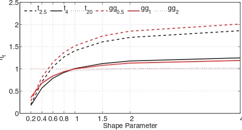
The scale parameter ηf is generic characteristic of non-Gaussian likelihoods and of the true innovations, and it does not change when using another conditional heteroscedastic model. Here, we numerically evaluate how it varies according to the non-Gaussian likelihoods and innovations.
Figures1and2show howηf varies over generalized Gaus-sian likelihoods and Student’st likelihoods with different pa-rameters, respectively. For each curve, which amounts to fixing a quasi-likelihood, the lighter the tails of innovation errors are, the largerηf. Furthermore,ηf >1 for innovation errors that are lighter than the likelihood, andηf <1 for innovations that are heavier than the likelihood. Therefore, if the non-Gaussian like-lihood has heavier tails than true innovation, we should shrink the estimates to obtain consistent estimates. On the other hand, if the quasi-likelihood is lighter than true innovation, we should magnify the estimates.
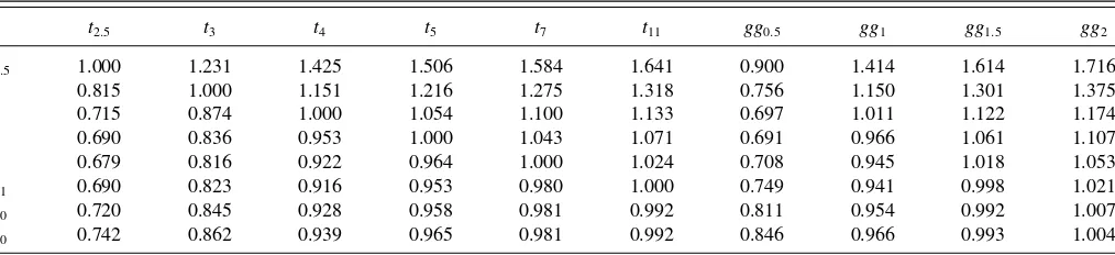
Tables1and2provide more values ofηf. For each column (fix an innovation distribution), in most cases the heavier the
0.2 0.4 0.6 0.8 1 1.5 2 4 0
0.5 1 1.5 2 2.5
ηf
Shape Parameter t
2.5 t4 t20 gg0.5 gg1 gg2
Figure 2. Variations ofηfacross generalized Gaussian innovations.
Table 1. ηffor generalized GQMLEs (gg,row) and innovation distributions (column)
gg0.2 gg0.6 gg1 gg1.4 gg1.8 gg2 t3 t5 t7 t11
gg0.2 1.000 6.237 8.901 10.299 11.125 11.416 8.128 9.963 10.483 10.885
gg0.6 0.271 1.000 1.291 1.434 1.515 1.544 1.159 1.384 1.443 1.487
gg1.0 0.354 0.844 1.000 1.073 1.114 1.128 0.900 1.040 1.074 1.098
gg1.4 0.537 0.873 0.962 1.000 1.022 1.029 0.883 0.977 0.998 1.012
gg1.8 0.811 0.952 0.981 0.993 1.000 1.002 0.946 0.985 0.991 0.997
tails of likelihoods are, the largerηf, but the monotone rela-tionship is not true for some ultra heavy-tail innovations, in which casesηf shows a “smile.” The nonmonotonicity in the likelihood dimension indicates that to determineηf one needs more information about the likelihood than just the asymptotic behavior of its tails. For example, both the true likelihood and Gaussian likelihood haveηf equal to 1.
7.2 Comparison With GQMLE, MLE, Rank, and Semiparametric Estimator
Here, we compare the efficiency of NGQMLE, GQMLE, MLE, and an adaptive estimator under various innovation error distributions. We fix the quasi-likelihood to be the Student’st distribution with a degree of freedom 7.
We include into the comparison the rank-based estimator by Andrews (2012). The estimator is obtained by minimizing the functionDT below:
DT(θ)= T
t=P+1 λ
Rt(θ)
T −p+1
(ξt(θ)−ξt(θ)),
where λ(·) is a nonconstant and nondecreasing function from (0,1) toR, Rt(θ) denotes the rank corresponding to ξt(θ)= log(ε2t(θ)), and ξt(θ)=(n−P)−1
T
t=P+1ξt(θ). We follow Andrews (2012) to choose λ(x) as {7(F−1
t7 ((x+1)/2))
2 −
5}/{(F−1
t7 ((x+1)/2))
2
+5}, where F−1
t7 represents the distri-bution function for rescaledt7 noise. The asymptotic relative
efficiency of the NGQMLE against the rank-based estimator is given in Table 3, with less-than-one ratios in favor of the NGQMLE. From this table, we can see that the two estima-tors are almost indistinguishable asymptotically with the rank-based estimator slightly better. This observation does not under-mine the appeal of the NGQMLE as it also estimates the scale parameter σ, and a by-product ηf, which gauges how large
the bias of non-Gaussian likelihood estimator is without scale adjustment.
We also consider the semiparametric estimator proposed by Drost and Klaassen (1997) in the setting of GARCH(1,1) with symmetric heavy-tailed errors. Their estimation is done in two steps. The first step runs a GQMLE to obtain estimates of pa-rameterθ =(a1,b1) as well as the noise series{εt}, with which they can construct the second-step estimator:
a1 b1
=
a1 b1
+
1 0 0 0 0 1 0 0
×
1
T
T
t=1
Wt(θ)t(ε)t(ε)′Wt(θ)′
−1
×1 T
T
t=1
Wt(θ)− 1
T
T
s=1
Ws(θ)
t(ε),
where
Wt(θ)=
⎛ ⎜ ⎝Ht(θ)
0,1
2v
−2 t (θ)
σ−1I 2
⎞ ⎟ ⎠,
Ht(θ)=βHt−1(θ)+
xt2−1 v2t−1(θ)
, H1(θ)=02×1,
t(ε)= −
l′(εt) 1+εtl′(εt)
, l′(ǫ)=g
′(εt)
g(εt)
, and
g(·)= 1 T
T
t=1
1
bT
K
· −εt
bT
.
Table 2. ηffor Student’stQMLEs (row) and innovation distributions (column)
t2.5 t3 t4 t5 t7 t11 gg0.5 gg1 gg1.5 gg2
t2.5 1.000 1.231 1.425 1.506 1.584 1.641 0.900 1.414 1.614 1.716
t3 0.815 1.000 1.151 1.216 1.275 1.318 0.756 1.150 1.301 1.375
t4 0.715 0.874 1.000 1.054 1.100 1.133 0.697 1.011 1.122 1.174
t5 0.690 0.836 0.953 1.000 1.043 1.071 0.691 0.966 1.061 1.107
t7 0.679 0.816 0.922 0.964 1.000 1.024 0.708 0.945 1.018 1.053
t11 0.690 0.823 0.916 0.953 0.980 1.000 0.749 0.941 0.998 1.021
t20 0.720 0.845 0.928 0.958 0.981 0.992 0.811 0.954 0.992 1.007
t30 0.742 0.862 0.939 0.965 0.981 0.992 0.846 0.966 0.993 1.004
Table 3. Asymptotic relative efficiency of Student’s 7 QMLEs against rank-based estimators
Student’st Generalized Gaussian
innovations ARE innovations ARE
t20 1.006 gg4 1.201
t9 0.998 Gauss. 1.027
t6 1.002 gg1 1.010
t4 1.025 gg0.8 1.029
t3 1.065 gg0.4 1.140
The choice of the first step estimation requires a finite fourth moment for the innovation. In our comparison, we chooseK(·) to be the Gaussian kernel, with a range of bandwidths equal to 0.1, 0.5, and 0.9, to demonstrate the effect of bandwidth selection in finite sample.
Our simulations are conducted using a GARCH(1,1) model with true parameters (σ, a1, b1)=(0.5,0.6,0.3). For innovation
errors we use Student’stand generalized Gaussian distributions of various degrees of freedoms and shape parameters to generate data. For each type of innovation distribution, we runN =1000 simulations each with sample size ranging among 250, 500, and
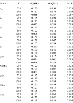
1000. Tables4,5, and6report the RMSE comparison of these three estimators.
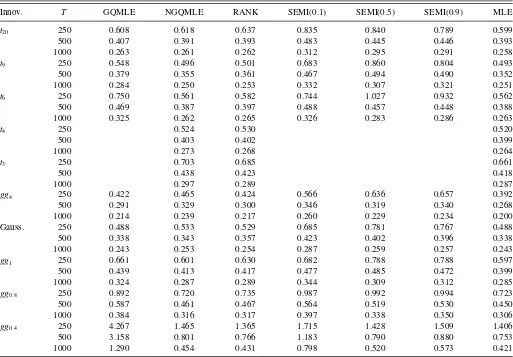
In the upper panel of Tables 4, 5, and 6, the innovation distributions range from thin-tailed t20 (approximately
Gaus-sian) to heavy-tailed t3. For the first thin-tailed t20 case,
GQMLE outperforms NGQMLE by a small margin. For all other cases, NGQMLE outperforms GQMLE. In the casest9
andt6, NGQMLE performs nearly as well as MLE, and reduces
standard deviations by roughly 20%–30% from GQMLE. In heavier tail cases (t4 andt3), since a fourth moment no longer
exists, GQMLE is not√T-consistent, and its estimation pre-cision quickly deteriorates, sometimes to an intolerable level. Hence, we omit reporting the estimates in the tables. In con-trast, NGQMLE using t4 likelihood does not require a finite
fourth moment for√T-consistenta1 andb1, so standard
de-viations fora1andb1 are still nearly equal to MLE. Standard
deviations ofσ are now larger than MLE, but still significantly smaller than GQMLE. The finite sample performance of the rank-based estimator is again indistinguishable compared to that of the NGQMLE, which agrees with the asymptotic relative effi-ciency inTable 3. The comparison with semiparametric estima-tor shows that the NGQMLE behaves better, especially in small sample, and the performance of the semiparametric estimator
Table 4. Comparison of RMSE ofa1with Student’stand generalized Gaussian innovations
Innov. T GQMLE NGQMLE RANK SEMI(0.1) SEMI(0.5) SEMI(0.9) MLE
t20 250 0.608 0.618 0.637 0.835 0.840 0.789 0.599
500 0.407 0.391 0.393 0.483 0.445 0.446 0.393
1000 0.263 0.261 0.262 0.312 0.295 0.291 0.258
t9 250 0.548 0.496 0.501 0.683 0.860 0.804 0.493
500 0.379 0.355 0.361 0.467 0.494 0.490 0.352
1000 0.284 0.250 0.253 0.332 0.307 0.321 0.251
t6 250 0.750 0.561 0.582 0.744 1.027 0.932 0.562
500 0.469 0.387 0.397 0.488 0.457 0.448 0.388
1000 0.325 0.262 0.265 0.326 0.283 0.286 0.263
t4 250 0.524 0.530 0.520
500 0.403 0.402 0.399
1000 0.273 0.268 0.264
t3 250 0.703 0.685 0.661
500 0.438 0.423 0.418
1000 0.297 0.289 0.287
gg4 250 0.422 0.465 0.424 0.566 0.636 0.657 0.392
500 0.291 0.329 0.300 0.346 0.319 0.340 0.268
1000 0.214 0.239 0.217 0.260 0.229 0.234 0.200
Gauss. 250 0.488 0.533 0.529 0.685 0.781 0.767 0.488
500 0.338 0.343 0.357 0.423 0.402 0.396 0.338
1000 0.243 0.253 0.254 0.287 0.259 0.257 0.243
gg1 250 0.661 0.601 0.630 0.682 0.788 0.788 0.597
500 0.439 0.413 0.417 0.477 0.485 0.472 0.399
1000 0.324 0.287 0.289 0.344 0.309 0.312 0.285
gg0.8 250 0.892 0.720 0.735 0.987 0.992 0.994 0.723
500 0.587 0.461 0.467 0.564 0.519 0.530 0.450
1000 0.384 0.316 0.317 0.397 0.338 0.350 0.306
gg0.4 250 4.267 1.465 1.365 1.715 1.428 1.509 1.406
500 3.158 0.801 0.766 1.183 0.790 0.880 0.753
1000 1.290 0.454 0.431 0.798 0.520 0.573 0.421
NOTE: We report the RMSE fora1in this table. The innovation errors followt-distribution with degrees of freedom equal to 20, 9, 6, 4, and 3, and generalized Gaussian distribution with
shape parameters equal to 4, 2, 1, 0.8, and 0.4, respectively. We follow Andrews (2012) to impose the constraintsa1>0 and 0< b1<1 in optimization. For semiparametric estimation,
we follow Drost and Klaassen (1997) to impose an additional constrainta1σ2+b1<1 in the first GQMLE step.
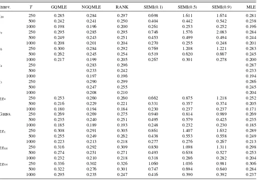
Table 5. Comparison of RMSE ofb1with Student’stand generalized Gaussian innovations
Innov. T GQMLE NGQMLE RANK SEMI(0.1) SEMI(0.5) SEMI(0.9) MLE
t20 250 0.285 0.284 0.297 0.698 1.611 1.674 0.281
500 0.242 0.241 0.250 0.404 0.442 0.542 0.238
1000 0.198 0.196 0.200 0.261 0.253 0.252 0.196
t9 250 0.295 0.285 0.295 0.746 1.576 2.083 0.284
500 0.249 0.243 0.251 0.453 0.499 0.494 0.244
1000 0.208 0.201 0.204 0.270 0.255 0.248 0.201
t6 250 0.300 0.284 0.292 0.769 1.208 1.221 0.283
500 0.262 0.245 0.254 0.519 0.620 0.667 0.245
1000 0.217 0.199 0.205 0.267 0.301 0.278 0.200
t4 250 0.283 0.296 0.287
500 0.233 0.242 0.233
1000 0.197 0.196 0.194
t3 250 0.290 0.299 0.286
500 0.247 0.255 0.245
1000 0.208 0.210 0.204
gg4 250 0.253 0.260 0.260 0.662 0.875 1.218 0.252
500 0.216 0.229 0.221 0.331 0.357 0.374 0.205
1000 0.180 0.194 0.184 0.230 0.237 0.237 0.171
Gauss. 250 0.269 0.269 0.275 0.940 0.814 0.989 0.269
500 0.235 0.240 0.251 0.495 0.579 0.425 0.235
1000 0.185 0.189 0.193 0.248 0.232 0.230 0.185
gg1 250 0.308 0.291 0.305 0.861 1.407 1.632 0.289
500 0.255 0.249 0.262 0.438 0.553 0.558 0.249
1000 0.223 0.213 0.218 0.277 0.276 0.267 0.213
gg0.8 250 0.316 0.292 0.309 0.850 1.098 1.311 0.298
500 0.274 0.251 0.271 0.493 0.638 0.527 0.253
1000 0.232 0.210 0.218 0.318 0.286 0.282 0.204
gg0.4 250 0.336 0.302 0.326 1.060 1.036 0.981 0.306
500 0.322 0.276 0.301 0.747 0.694 0.640 0.284
1000 0.295 0.235 0.247 0.416 0.390 0.392 0.237
varies with the choice of the bandwidth. The semiparametric estimator is clearly less attractive compared to the NGQMLE, since the NGQMLE is free of tuning parameters, and its gap in efficiency (compared to MLE) is not large at all.
In the lower panel, the innovations range from thin tailed
gg4to heavy-tailedgg0.4. For innovations withgg1and heavier,
NGQMLE starts to outperform GQMLE, and in all such cases, the Studentt7NGQMLE performs very close to MLE. In
com-parison, GQMLE’s performance deteriorates as tails grow heav-ier, particularly ingg0.8 andgg0.4, although in these cases the
fourth moments are finite. The comparison results with the rank-based estimator, the semiparametric estimator, and the MLE are similar to the cases with Student’stinnovations.
8 EMPIRICAL WORK
To demonstrate the empirical relevance of our approach, we estimate values ofηf for S&P 500 components. To do so, we fit GARCH(1,1) models to daily returns collected from January 2, 2004, to December 30, 2011, so the sample contains 2015 trading days in total. There are 458 stocks selected from the current S&P 500 stocks, as they have been traded since the beginning of the sample. We apply two common likelihood functions that are extensively used in the literature, including Student’stlikelihood with degree of freedom 4, and generalized
Gaussian likelihood with shape parameter equal to 1.Figure 3 provides an illustration of the empirical distributions of their respectiveηf’s. It is clear from the plot that most stocks have
ηf’s larger than 1, indicating the tail in the data is less heavier than the likelihoods we select. On the other hand, most ηf’s deviate from 1 by a wide margin, showing that the bias of likelihood estimates without adjustments could be as large as 15%–20%. In summary, the message we want to deliver here is the extra step ofηf adjustment is necessary for non-Gaussian likelihood estimators.
0.750 0.8 0.85 0.9 0.95 1 1.05 1.1 1.15 1.2 1.25 20
40 60
Student t4 Likelihood
0.750 0.8 0.85 0.9 0.95 1 1.05 1.1 1.15 1.2 1.25 50
100
Generalized Gaussian gg1 Likelihood
Figure 3. Empirical estimates ofηf across S&P 500 component
stocks.
Table 6. Comparison of RMSE ofσwith Student’stand generalized Gaussian innovations
Innov. T GQMLE NGQMLE MLE
t20 250 0.130 0.130 0.128
500 0.111 0.110 0.109
1000 0.088 0.087 0.087
t9 250 0.135 0.128 0.128
500 0.113 0.110 0.110
1000 0.093 0.088 0.088
t6 250 0.145 0.133 0.132
500 0.122 0.112 0.112
1000 0.095 0.086 0.087
t4 250 0.150 0.134 0.131
500 0.129 0.107 0.102
1000 0.107 0.089 0.084
t3 250 0.230 0.171 0.132
500 0.170 0.148 0.109
1000 0.138 0.103 0.088
gg4 250 0.114 0.117 0.112
500 0.094 0.101 0.088
1000 0.078 0.085 0.073
Gauss. 250 0.122 0.122 0.122
500 0.104 0.107 0.104
1000 0.081 0.083 0.081
gg1 250 0.147 0.135 0.134
500 0.116 0.113 0.113
1000 0.100 0.095 0.095
gg0.8 250 0.153 0.139 0.140
500 0.127 0.114 0.115
1000 0.105 0.093 0.090
gg0.4 250 0.189 0.163 0.149
500 0.172 0.142 0.135
1000 0.148 0.110 0.106
NOTE: We report the RMSE forσin this table. The innovation errors followt-distribution with degrees of freedom equal to 20, 9, 6, 4, and 3, and generalized Gaussian distribution with shape parameters equal to 4, 2, 1, 0.8, and 0.4, respectively.
9 CONCLUSION
This article focuses on GARCH model estimation when the innovation distribution is unknown, and it questions the effi-ciency of GQMLE and consistency of the popular NGQMLE. It proposes the NGQMLE to tackle both issues. The first step of the proposed procedure runs a GQMLE whose purpose is to identify the unknown scale parameterηfin the second step. The final step performs an NGQMLE to estimate model parameters. The quasi-likelihoodf can be a prespecified heavy-tailed likeli-hood, properly scaled byηfor selected from a pool of candidate distributions.
The asymptotic theory of NGQMLE does not depend on any symmetric or unimodal assumptions of innovations. By adopting the different parameterization proposed by Newey and Steigerwald (1997), and incorporatingηf, NGQMLE improves the efficiency of GQMLE. This article shows that the asymp-totic behavior of NGQMLE can be broken down to two parts. For the heteroscedastic parameterγ, NGQMLE is always√T -consistent and asymptotically normal, whereas√T-consistency of GQMLE relies on finite fourth moment assumption. When
Eε4
t <∞, NGQMLE outperforms GQMLE in terms of smaller asymptotic variance, provided that innovation distribution is
rea-sonably heavy-tailed, which is common for financial data. For the scale partσ, NGQMLE is not always√T-consistent. The article also provides simulations to compare the performance of GQMLE, NGQMLE, semiparametric estimator, and MLE. In most cases, NGQMLE shows an advantage and is close to the MLE.
A. APPENDIX
A.1 Proof of Lemma 1
Proof. Note that
Et(l(x¯t,θ))=Q
ηfσ vt(γ)
σ0vt(γ0)
−logσ0vt(γ0)+logηf
≤Q(ηf)−logσ0vt(γ0)+logηf
=Et(l(x¯t,θ0)).
Also, Assumption 1 implies that if vt(γ)=vt(γ0) a.s., then
γ =γ0, see for example, (Francq and Zako¨ıan2004, p. 615).
By Assumption 2, the inequality holds with positive probability. Therefore, by iterated expectations, ¯L(θ)<L¯(θ0).
A.2 Proof of Theorem 1
Proof. It is straightforward to verify that (θ0, ηf,θ0) satisfy
the following equation:
E(s(x¯t,θ, η,φ))=0,
Assumptions 1 and 2 guarantee the uniqueness, hence iden-tification is established. By Theorem 2.6 in Newey and Mc-Fadden (1994) (a generalized version for stationary and er-godicxt), along with Assumption 3 (ii), we have the desired
consistency.
A.3 Proof of Proposition 1
Proof. Define the likelihood ratio function G(η)=
E(log( 1
ηf( ε η)
f(ε) )). SupposeG(η) has no local extremal values. And
since log(x)≤2(√x−1),
E
log
1
ηf( ε η)
f(ε)
≤2E
⎛ ⎝
1
ηf( ε η)
f(ε) −1
⎞ ⎠
=2
+∞
−∞
1
ηf
x η
f(x)dx−2
≤ −
+∞
−∞
1
ηf
x η
−f(x)
2 dx
≤0.
The equality holds if and only ifη=1. Therefore,η=1 is the
unique maximum ofQ(η).
A.4 Proof of Theorem 2
To show the asymptotic normality, we first list some no-tations and derive a lemma. For convenience, we denote
y0= v1
var(y0)−1. All the expectations above are taken under the true
densityg. Note that from Section3.2, we have
s1( ¯xt,θ)=
First, we need a lemma.
Lemma 2. The following claims hold:
1. The inverse ofMin block expression is
M−1=
unit column vector that has the same length as θ, with the first entry one and all the rest zeros.
Proof. The proof uses Moore–Penrose pseudo inverse de-scribed in Ben-Israel and Greville (2003). Observe that
M =
Using the technique of Moore–Penrose pseudo inverse, we have
M−1=
whereHis formed by the elements below:
β =1+¯y′0V¯y0, w=
So Equation (A.7) is obtained by plugging H into Equation (A.9). The rest two points of the lemma can be obtained by
simple matrix manipulation.
Next we return to the proof of Theorem 2.
Proof. According to Theorem 3.4 in Newey and McFadden (1994) (a generalized version for stationary and ergodic xt), (θT,η,θT) are jointly T
1
2-consistent and asymptotic normal.
The asymptotic variance matrix is
G−1Es(x¯t,θ0, ηf,θ0)s(x¯t,θ0, ηf,θ0)′
G′−1, (A.10)
where G=E(∇s(x¯t,θ0, ηf,θ0)). View this matrix as 3×3
blocks, with asymptotic variances of (θT,η,θT) on the first, second, and third diagonal blocks. We now calculate the second and third diagonal blocks. The expected Jacobian matrixGcan be decomposed into
The second diagonal block depends on the second row ofG−1
ands(x¯t,θ0, ηf,θ0). The second row ofG−1is
The last step uses the second point of Lemma 2. So Equation (15) is obtained by plugging in the expressions forG22andq2.
The last step uses the second point of Lemma 2. Then
Eq3q3′
Therefore, Equation (14) is obtained by plugging in the ex-pressions for G33, Eq3q3′, and apply the third point of
Lemma 2.
Note that in the case where ηf is known, the asymptotic variance ofθis
The asymptotic covariance between θ and ηf is G33−1E(q3q2)G′−221. A direct calculation using the second point
of Lemma 2 yields
=ηfσ0
The same formula recurs in the asymptotic covariance between
θandηf, which isG11−1E(q1q2)G′−221.
Finally, the asymptotic covariance between θ and θ is G11−1E(q1q′3)G33′−1, denoted as. It implies from the third
point of Lemma 2 that
= E(h1(ε, ηf)(1−ε
which concludes the proof.
A.5 Proof of Theorem 3
Proof. Following the similar idea to GMM, we may prove:
⎛
Thus, the submatrices corresponding to γ parameter are 0’s. Therefore, the first step has no effect on the central limit theorem
ofγT. The result follows from Lemma 2. In terms ofσT, its convergence rate becomesT λ−T1.
A.6 Proof of Proposition 2
Proof. Denote by random variables κG=(1−ε2)/2, and
Therefore, we obtainw∗
1 =E(κG(κG+κ2))/E(κG+κ2)2. Now
Therefore, all the optimal aggregation weights are the same. The optimal variance follows from direct calculations. Note that the estimation of ω∗ does not lead to a larger asymp-totic variance because θ∗T −(W∗θ+(I−W∗)θ)=(W∗−
We are grateful for helpful suggestions from the editor, the associated editor and the referees, extensive discussions with Chris Sims and Enrique Sentana, and thoughtful comments from seminar and conference participants at Princeton Uni-versity, the 4th CIREQ Time Series Conference, and the 10th World Congress of the Econometric Society. Financial support from NSF Grant DMS-0704337 and DMS-1206464, and the University of Chicago Booth School of Business is gratefully acknowledged.
[Received November 2012. Revised March 2013.]
REFERENCES
Andrews, B. (2012), “Rank-Based Estimation for GARCH Processes,” Econo-metric Theory, 28, 1037–1064. [179,185]
Ben-Israel, A., and Greville, T. (2003),Generalized Inverses Theory and Appli-cations, New York: Springer. [189]
Berkes, I., and Horv´ath, L. (2004), “The Efficiency of the Estimators of the Parameters in Garch Processes,”The Annals of Statistics, 32, 633–655. [179]
Berkes, I., Horv´ath, L., and Kokoszka, P. (2003), “Garch Processes: Structure and Estimation,”Bernoulli, 9, 201–227. [178,180]
Bollerslev, T. (1986), “Generalized Autoregressive Conditional Heteroskedas-ticity,”Journal of Econometrics, 31, 307–327. [178]
——— (1987), “A Conditionally Heteroskedastic Time Series Model for Spec-ulative Prices and Rates of Return,”The Review of Economics and Statistics, 69, 542–547. [178]
Bollerslev, T., and Wooldbridge, J. M. (1992), “Quasi-maximum Likelihood Estimation and Inference in Dynamic Models With Time-varying Covari-ances,”Econometric Reviews, 11, 143–172. [178,179]
Bougerol, P., and Picard, N. (1992), “Stationarity of Garch Processes and of Some Nonnegative Time Series,”Journal of Econometrics, 52, 115–127. [179]
Diebold, F. (1988),Empirical Modeling of Exchange Rate Dynamics, New York: Springer. [178]
Drost, F. C., and Klaassen, C. A. J. (1997), “Efficient Estimation in Semiparametric Garch Models,”Journal of Econometrics, 81, 193–221. [178,179,183,185]
Elie, L., and Jeantheau, T. (1995), “Consistency in Heteroskedastic Mod-els,” Comptes Rendus de l ’Acad´emie des Sciences, 320, 1255– 1258. [178]
Engle, R. F. (1982), “Autoregressive Conditional Heteroscedasticity With Es-timates of the Variance of United Kingdom Inflation,”Econometrica, 50, 987–1007. [178]
Engle, R. F., and Bollerslev, T. (1986), “Modelling the Persistence of Conditional Variances,”Econometric Reviews, 5, 1–50. [178]
Engle, R. F., and Gonzalez-Rivera, G. (1991), “Semiparametric Arch Models,”
Journal of Business and Economic Statistics, 9, 345–359. [178]
Fiorentini, G., and Sentana, E. (2010), “On the Efficiency and Consistency of Likelihood Estimation in Multivariate Conditionally Heteroskedastic Dy-namic Regression Models,” unpublished manuscript, CEMFI. [181] Francq, C., Lepage, G., and Zako¨ıan, J.-M. (2011), “Two-stage Non Gaussian
QML Estimation of GARCH Models and Testing the Efficiency of the Gaussian QMLE,”Journal of Econometrics, 165, 246–257. [179,181,182] Francq, C., and Zako¨ıan, J.-M. (2004), “Maximum Likelihood Estimation of
Pure GARCH and ARMA-GARCH Processes,”Bernoulli, 10, 605–637. [188]
Gonz´alez-Rivera, G., and Drost, F. C. (1999), “Efficiency Comparisons of Maximum-likelihood-based Estimators in Garch Models,”Journal of Econometrics, 93, 93–111. [178,183]
Hall, P., and Yao, Q. (2003), “Inference in Arch and Garch Models With Heavy-tailed Errors,”Econometrica, 71, 285–317. [178,180,183]
Hsieh, D. A. (1989), “Modeling Heteroscedasticity in Daily Foreign-Exchange Rates,”Journal of Business and Economic Statistics, 7, 307–317. [178]
Huang, D., Wang, H., and Yao, Q. (2008), “Estimating GARCH Models: When to Use What?,”Econometrics Journal, 11, 27–38. [179]
Lee, S.-W., and Hansen, B. E. (1994), “Asymptotic Theory for the Garch (1, 1) Quasi-maximum Likelihood Estimator,”Econometric Theory, 10, 29–52. [178]
Lee, T., and Lee, S. (2009), “Normal Mixture Quasi-maximum Likelihood Estimator for GARCH Models,”Scandinavian Journal of Statistics, 36, 157–170. [179,181]
Linton, O. (1993), “Adaptive Estimation in Arch Models,”Econometric Theory, 9, 539–569. [178]
Lumsdaine, R. L. (1996), “Consistency and Asymptotic Normality of the Quasi-maximum Likelihood Estimator in Igarch(1, 1) and Covariance Stationary Garch(1, 1) Models,”Econometrica, 64, 575–596. [178]
Nelson, D. B. (1991), “Conditional Heteroskedasticity in Asset Returns: A New Approach,”Econometrica, 59, 347–370. [178]
Newey, W. K., and McFadden, D. (1994), “Large Sample Estimation and Hy-pothesis Testing,” inHandbook of EconometricsVol. 4 , chap. 36, eds. R. F. Engle and D. McFadden, North Holland: Elsevier, pp. 2111–2245. [188,189]
Newey, W. K., and Steigerwald, D. G. (1997), “Asymptotic Bias for Quasi-maximum-likelihood Estimators in Conditional Heteroskedasticity Mod-els,”Econometrica, 65, 587–599. [179,180,181,188]
Peng, L., and Yao, Q. (2003), “Least Absolute Deviations Estimation for ARCH and GARCH Models,”Biometrika, 90, 967–975. [179]
Sun, Y., and Stengos, T. (2006), “Semiparametric Efficient Adaptive Estimation of Asymmetric GARCH Models,”Journal of Econometrics, 133, 373–386. [178]
Weiss, A. A. (1986), “Asymptotic Theory for Arch Models: Estimation and Testing,”Econometric Theory, 2, 107–131. [178]
White, H. (1982), “Maximum Likelihood Estimation of Misspecified Models,”
Econometrica, 50, 1–26. [180]
Comment
Beth A
NDREWSDepartment of Statistics, Northwestern University, Evanston, IL 60208 ([email protected]; [email protected])
In their article, Fan, Qi, and Xiu develop non-Gaussian quasi-maximum likelihood estimators (QMLEs) for the parameters θ=(σ,γ′)′=(σ, a
1, . . . , ap, b1, . . . , bq)′of a generalized au-toregressive conditional heteroscedasticity (GARCH) process
{xt}, where
xt =σ vtεt,
vt2=1+
p
i=1
aixt2−i+ q
j=1 bjvt2−j,
and the noise {εt}are assumed to be independent and iden-tically distributed with mean zero and variance one. The QMLEs ofγare shown to be√T-consistent (Trepresents sam-ple size) and asymptotically Normal under general conditions. When E{ε4
t}<∞, the QMLEs of the scale parameterσare also
√
T-consistent and asymptotically Normal, but, as is the case for Gaussian QMLEs of GARCH model parameters, the estimator ofσ has a slower rate of convergence otherwise (Hall and Yao 2003). As Fan, Qi, and Xiu mention, a rank-based technique for estimatingθwas presented in Andrews (2012). These rank (R
)-estimators are also consistent under general conditions, with the same rates of convergence as the non-Gaussian QMLEs. Hence, theR-estimators have robustness properties similar to the QMLEs. In this comment, I make some methodological and efficiency comparisons between the two techniques, and suggest R-estimation be used prior to QMLE for preliminary GARCH estimation. Once anR-estimate has been found, corresponding model residuals can be used to identify one or more suitable noise distributions and QMLE/MLE can then be used. As Fan, Qi, and Xiu suggest in Section 6, one can optimize over a pool of appropriate likelihoods in an effort to improve efficiency. Ad-ditionally, MLEs of all elements ofθ are consistent with rate
√
T under general conditions (Berkes and Horv´ath2004).
© 2014American Statistical Association Journal of Business & Economic Statistics April 2014, Vol. 32, No. 2 DOI:10.1080/07350015.2013.875921