Full Terms & Conditions of access and use can be found at
http://www.tandfonline.com/action/journalInformation?journalCode=ubes20
Download by: [Universitas Maritim Raja Ali Haji] Date: 13 January 2016, At: 00:33
Journal of Business & Economic Statistics
ISSN: 0735-0015 (Print) 1537-2707 (Online) Journal homepage: http://www.tandfonline.com/loi/ubes20
Regime Shifts, Risk Premiums in the Term
Structure, and the Business Cycle
Ravi Bansal, George Tauchen & Hao Zhou
To cite this article: Ravi Bansal, George Tauchen & Hao Zhou (2004) Regime Shifts, Risk
Premiums in the Term Structure, and the Business Cycle, Journal of Business & Economic Statistics, 22:4, 396-409, DOI: 10.1198/073500104000000398
To link to this article: http://dx.doi.org/10.1198/073500104000000398
View supplementary material
Published online: 01 Jan 2012.
Submit your article to this journal
Article views: 106
View related articles
Regime Shifts, Risk Premiums in the Term
Structure, and the Business Cycle
Ravi B
ANSALFuqua School of Business, Duke University, Durham, NC 27708 (rb7@mail.duke.edu)
George T
AUCHENDepartment of Economics, Duke University, Durham, NC 27708 (get@econ.duke.edu)
Hao Z
HOUFederal Reserve Board, Washington, DC 20551 (hao.zhou@frb.gov)
Recent evidence indicates that using multiple forward rates sharply predicts future excess returns on U.S. Treasury Bonds, with theR2’s being around 30%. The projection coefficients in these regressions exhibit a distinct pattern that relates to the maturity of the forward rate. These dimensions of the data, in conjunction with the transition dynamics of bond yields, offer a serious challenge to term structure models. In this article we show that a regime-shifting term structure model can empirically account for these challenging data features. Alternative models, such as affine specification, fail to account for these important features. We find that regimes in the model are intimately related to bond risk premia and real business cycles.
KEY WORDS: Business cycle; Efficient method of moments; Expectation hypothesis; Regime shifting; Term structure of interest rate.
1. INTRODUCTION
Term structure models with regime shifts, considered by Naik and Lee (1997) and Bansal and Zhou (2002), capture the important feature that the aggregate economy is subject to discrete and persistent changes in the business cycle. The business cycle fluctuations, together with the monetary policy response to them, have significant impacts not only on the short-term interest rate, but also on the entire short-term structure. Regime-shifting term structure models represent a parsimonious way of introducing interactions between the business cycles, the term structure, and risk premia on bonds. Using the U.S. Treasury yield data from 1964 to 1995, Bansal and Zhou (2002) found that the model-implied regime changes usually lead or coin-cide with economic recessions. Therefore, the term structure regimes seem to confirm and complement the real business cy-cles. This evidence also allows for the possibility that this class of term structure models may be able to capture the dynamics of risk premia on bonds.
The most common strategy for understanding bond risk pre-miums is to study deviations from the expectations hypothesis. One form of the violation, that the regression of yield changes on yield spreads produces negative slope coefficient instead of unity (Campbell and Shiller 1991), has been addressed in many recent articles (e.g., Roberds and Whiteman 1999; Dai and Singleton 2002; Bansal and Zhou 2002; Evans 2003). An-other form of violation of the expectations hypothesis is that the forward rate can predict the excess bond return (Fama and Bliss 1987). More recently, Cochrane and Piazzesi (2002) doc-umented that using multiple forward rates to predict bond ex-cess returns generates very high predictability of bond exex-cess returns, with adjustedR2’s from the regression of around 30%. Further, they showed that the coefficients of multiple forward-rate regressors form a tent-shaped pattern related to the maturity of the forward rate. The size of the predictability and nature of projection coefficients is quite puzzling and constitutes a chal-lenge to term structure models.
The main contribution of this article is to account for the predictability evidence from the perspective of latent factor term structure models. When evaluating the plausibility of var-ious term structure models, it is important to not focus ex-clusively on the predictability issue; previous work (e.g., Dai and Singleton 2000; Bansal and Zhou 2002; Ahn, Dittmar, and Gallant 2002) highlights the difficulties that many received models have in capturing the transition dynamics of yields (i.e., conditional volatility and conditional cross-correlation across yields). The predictability evidence, in conjunction with the transition dynamics, constitutes a sufficiently rich set of data features for discriminating across alternative term structure models and to evaluate their plausibility. The main empirical finding of this article is that the regime-shifting term struc-ture models can simultaneously justify the size and nastruc-ture of bond return predictability and the transition dynamics of yields. More specifically, we find that models with regime shifts can re-produce the high predictability and the tent-shaped regression coefficients documented by Cochrane and Piazzesi (2002). Ad-ditionally, the regime-shifting term structure model reproduces the dynamics of conditional volatility and cross-correlation across yields. In contrast, commonly used multifactor Cox– Ingersoll–Ross (CIR) (Cox, Ingersoll, and Ross 1985) and affine models cannot capture these dimensions of the data. Our overall evidence indicates that incorporating regime shifts is important for interpreting key aspects of Treasury bond market data.
We use U.S. Treasury yield data from 1964–2001. The pe-riod 1996–2000 poses a tough challenge for standard asset pricing models, with unprecedented long economic growth and bull market run. At the same time, this period includes several economic recessions and periods of economic boom.
In the Public Domain Journal of Business & Economic Statistics October 2004, Vol. 22, No. 4 DOI 10.1198/073500104000000398 396
Using the whole sample, we find that the conditional corre-lation between the long and short yields vary over a range of about 40–80%. The conditional volatilities of the long and short yields also reveal very large variations. Despite this, when evaluating the U.S. Treasury yields data from 1964–2001, our regime-shifting model still stands out as the best-performing candidate. The regime indicator is related to business cycles in the data; for example, the model-based regime indicator pre-dicts the 2001–2002 recession.
To estimate various models under consideration, we use the efficient method of moments (EMM), developed by Bansal, Gallant, Hussey, and Tauchen (1995) and Gallant and Tauchen (1996). Tests of overidentifying restrictions based on the EMM method provide a way to compare different, potentially nonnested models. This estimation technique forces the model to confront several important aspects of the data, such as con-ditional volatility and correlation across different yields. To generate diagnostic evidence to help discriminate across mod-els, we rely on the reprojection methods developed by Gallant and Tauchen (1998). Our empirical evidence suggests that the benchmark CIR and affine model specifications with up to three factors are sharply rejected withp values of 0. The only model specification that finds support in the data (withpvalue of 1%) is our preferred two-factor regime-switching model, where the market prices of risks depend on regime shifts. Our diagnostics of the various models show that the our pre-ferred regime-shifting model specification produces the small-est cross-sectional pricing errors across all of the specifications we considered. Using reprojections, we computed the condi-tional correlations and volatility under the null of the various models. Our results show that only the regime-shifting models can capture the large variations in conditional correlations and conditional volatility that are observed in the data.
The article is organized as follows. Section 2 reviews the regime-shifting term structure model developed by Bansal and Zhou (2002). Section 3 discusses the empirical estimation re-sults, the specification tests, and an array of diagnostics based on the conditional correlation and volatility. It also examines cross-sectional implications on pricing errors, violations of the expectation hypothesis of forward rate predictability, and the link between regime classification and business cycles, espe-cially the recent economic recession. Section 4 presents some concluding remarks.
2. TERM STRUCTURE MODEL WITH REGIME SHIFTS
In this section we review the term structure model with regime shifts proposed by Bansal and Zhou (2002). The deriva-tion focuses on a single-factor specificaderiva-tion; the multifactor extension is straightforward (see Bansal and Zhou 2002). To capture the idea that the aggregate economy is subject to regime shifts, we model the regime-shifting process as a two-state Markov process, as was done by Hamilton (1989). Suppose that the evolution of tomorrow’s regime,st+1=0,1, given today’s regime,st=0,1, is governed by the transitional probability ma-trix of a Markov chain,
= discrete regime shifts, the economy is also affected by a continuous-state variable, reversion, long-run mean, and volatility parameters. All of these parameters are subject to discrete regime shifts. Specif-ically, Xt+1−Xt =κ0(θ0−Xt)+σ0√Xtut+1 if the regime
st+1=0, and Xt+1−Xt =κ1(θ1−Xt)+σ1√Xtut+1 if the regimest+1=1. Note that the innovation in process (2),ut+1, is conditionally normal givenXtandst+1. For analytical tractabil-ity we assume that the process for regime shiftsst+1is indepen-dent ofXt+1−l,l=0, . . . ,∞, this is similar to the assumptions made in Hamilton’s regime-switching models. We also assume that the agents in the economy observe the regimes, although the econometrician may possibly not observe the regimes.
The pricing kernel for this economy is similar to that in stan-dard models, except for incorporating regime shifts,
Mt+1=exp
The foregoing specification of the pricing kernel captures the intuition that these aggregate processes are latent and subject to regime shifts (as in Hamilton 1989). Note that theλparameter that affects the risk premia on bonds is also subject to regime shifts and hence depends onst+1. Bansal and Zhou (2002) pre-sented a general equilibrium model that leads to the pricing ker-nel in (3).
With regime shifts, we conjecture that the bond price with
n periods to maturity at date t depends on the regimest=i,
i=0,1, andXt
Pi(t,n)=exp{−Ai(n)−Bi(n)Xt}.
The one-period-ahead bond price, analogously, depends on
st+1andXt+1,
In addition, we impose the boundary condition Ai(0) =
Bi(0)=0 and the normalization Ai(1)=0, Bi(1)=1, for The conditional mean and volatility of the bond return in regime
st+1 are µn,st+1,t and σ 2
n,st+1,t. Equation (4) captures the idea that all risk premia and bond prices at datet depend only on
st andXt. To gain further intuition regarding this risk premium result, note that−σst+1Bst+1(n−1)
Xt]is the exposure of the pricing kernel tout+1in regimest+1. The covariance between these exposures determines the compensation for risk in regimest+1. Hence the risk compensation for regimest+1is the product
−σst+1Bst+1(n−1)
Given information regardingst,Xt, and the regime transition probabilities, agents integrate out the future regime,st+1, which leads to the risk premium result stated in (4). In the absence of regime shifts, the risk premium in (4), would simply be
−XtB(n−1)λ. Hence incorporating regime shifts makes the “beta” of the asset (i.e., the coefficient onXt) be time varying and dependent on the current regime. This fashion of making the asset “beta” time varying is potentially important for cap-turing the behavior of risk premia on bonds. In this model the market price of risk (i.e., the risk premium for an asset with a unit exposure tout+1) isEt[λst+1/σst+1|st]
√
Xt, which is clearly regime dependent.
Given (4), the solution for the bond prices can be derived by solving for the unknown coefficientsAandB. In particular,
Note that bond price coefficients are mutually dependent on both regimes; current bond prices reflect the agent’s expecta-tions regarding regime shifts in the future. Finally, the bond yield of aKfactor regime-shifting model can be derived in an analogous manner,
The foregoing regime-shifting term structure model does not entertain the possibility of separate risk compensation for regime shifts. In other words, the risk premium for a security that pays 1 dollar contingent on a regime shift at date t+1 is 0. The model can be extended to include explicit and sepa-rate compensation for regime-shifting risks. Such an extension entails additional parameters, however. We have not discussed or pursued this more embellished version of the model, because we found identifying and estimating its parameters very diffi-cult. Further, as documented later, the key puzzles in the term structure data, can be accounted for by the more parsimonious model described earlier.
Dai, Singleton, and Yang (2003) recently incorporated a sep-arate risk premium for regime-shifts but, for analytical tractabil-ity, assumed that the within-regime volatility is constant. Given the nature of yields data, it would seem that allowing within-regime volatility to be stochastic is quite important. It remains to be seen whether the specification that assumes a constant within-regime volatility can account for the observed time-varying volatility and conditional cross-correlation of yields. As discussed in the next section in our empirical work, these dimensions of the term structure data are important in discrim-inating across term structure models.
3. EMPIRICAL ESTIMATION AND MODEL EVALUATION
3.1 Estimation Methodology
To utilize a consistent approach for evaluation and estimation across the different models, we rely on the simulation-based EMM estimator developed by Bansal et al. (1995) and Gallant and Tauchen (1996). The EMM estimator comprises three steps. The first, the projection step, entails estimating a reduced-form model (the auxiliary model) that provides a good statisti-cal description of the data. Multivariate bond yields are difficult data to model, because they exhibit extreme persistence in lo-cation and scale, time-varying correlations, and non-Gaussian innovations. Because we do not have good a priori information on the specifications of a model that captures all of these fea-tures, we utilize a seminonparametric (SNP) series expansion. The SNP expansion has a vector autoregressive–autoregressive conditional heteroscedasticity (VAR–ARCH) Gaussian density as its leading term, and the departures from the leading term are captured by a Hermite polynomial expansion. We elected to use a simpler, ARCH-like leading term instead of a gener-alized ARCH (GARCH)-type leading term because of the sim-ilar problems with multivariate GARCH-type models of bond yields noted by Ahn et al. (2002).
In the second step, the estimation step, the score function from the log-likelihood estimation of the auxiliary model is used to generate moments for a generalized method of moments (GMM)-type criterion function. The score function provides a set of moment conditions that are true by construction and are to be confronted by all term structure models under consider-ation. In the computations, the score function is averaged over the simulation output from a given term structure model and the criterion function is minimized with respect to the parame-ters of the term structure model under consideration. By using the scores from the nonparametric SNP density as the moment conditions, each model is forced to match the conditional dis-tribution of the observed 6-month and 5-year yields. Being a GMM-type estimator, EMM provides a chi-squared measure of goodness of fit. In particular, the normalized objective function acts as an omnibus specification test, which is distributed as a chi-squared test (as in GMM) with degrees of freedom equal to the number of scores (moment conditions) minus the number of parameters in the particular term structure model. The distance matrix (the weight matrix in GMM) used in constructing the specification test is identical across different model specifica-tions (the null hypotheses). Consequently, thepvalues based on this specification test can be directly compared across different structural models to identify the best model specification. (For a discussion of the importance of having the same distance ma-trix, for a consistent comparison across models, see Hansen and Jagannathan 1997.) It is well recognized in the literature that tests for the absence of regime shifts against a regime-shifting alternative require nonstandard approaches (see Hansen 1992; Garcia 1998). Our approach of comparing all the considered models to a common nonparametric density (the SNP density), allows us to rank order all of the considered models according to the p values implied by the EMM criterion function. The advantage of using the nonparametric SNP (as discussed by Gallant and Tauchen 1999), is that it can asymptotically
Table 1. Summary Statistics
1-month 3-month 6-month 1-year 2-year 3-year 4-year 5-year
Mean 5.9424 6.3765 6.5971 6.8106 7.0156 7.1711 7.2909 7.3545
Standard deviation 2.4499 2.5767 2.6038 2.5239 2.4559 2.3814 2.3491 2.3240
Skewness 1.4278 1.3717 1.3041 1.1737 1.1288 1.1283 1.1003 1.0565
Kurtosis 5.4659 5.1336 4.8778 4.4157 4.1226 4.0313 3.9196 3.7344
NOTE: There are 451 monthly observations of the yields with 8 maturities. The data are obtained from CRSP Treasury Bill and Bond files, ranging from June 1964 to December 2001.
verge to virtually any smooth distributions, including mixture distributions (as is the case with a model of regime shifts).
The third step is reprojection, or postestimation analysis of model simulations. Because EMM is a simulation-based esti-mator, long simulated realizations from each estimated model are available for analysis. These simulations can be used to compute statistics of interest that can be compared to analo-gous values computed from the observed data. The reprojected statistics should be thought of as population quantities implied by the model at the estimated parameter values. Among other things, we compute the reprojected Cochrane–Piazzesi forward rate regressions for models with and without regime shifting.
3.2 Data Description
The dataset comprises monthly (June 1964–December 2001) bond yield data obtained from the Center for Research in Se-curity Prices (CRSP). There are a total of 451 monthly obser-vations with 8 maturities: 1-, 3-, and 6-month and 1-, 2-, 3-, 4-, and 5-year. It is important to recognize that the data period 1964–2001 contains six major recessions and six major
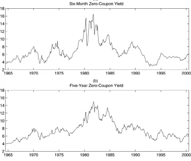
expan-sions, which, as stated earlier, provides potential economic mo-tivation for incorporating regime shifts. The summary statistics of these monthly yields are displayed in Table 1. On average, the yield curve is upward sloping. The standard deviation, pos-itive skewness, and kurtosis are systematically higher for short maturities than for long ones. To incorporate important time se-ries and cross-sectional aspects of term structure data, we focus on a short-term yield and a long-term yield, the yields on the 6-month bill and the 5-year note. Time series plots of the basis yields are shown in Figure 1. It is not unusual for using two or three time series to estimate a model with three or more latent factors, because the identification is coming from the number of scores (or moment restrictions) generated from the auxil-iary model (see, e.g., Chernov, Gallant, Ghysels, and Tauchen 2003).
We very briefly summarize the first step estimation results for the nonparametric SNP specification, which was guided by the BIC information criterion; details are available on re-quest. The leading term of the bivariate SNP density has one lag in the VAR-based conditional mean (Lµ=1) and five lags
(a)
(b)
Figure 1. Observed Short-Term (a) and Long-Term (b) Rates.
in ARCH specification (Lr=5). The preferred specification ac-commodates departures from conditional normality via a Her-mite polynomial of degree 4 (Kz=4). This “semiparametric ARCH” specification is similar to that proposed by Engle and González-Rivera (1991) and allows for skewness and kurtosis in the error distribution. The total number of parameters for the specification isla=28; hence each model must confront a total of 28 data-determined moment conditions.
The conditional moments of the estimated SNP density for the observed interest rates are available analytically. It is fairly instructive to focus on some specific aspects of the estimated nonparametric SNP bivariate density. The top panel in Figure 6 (Sec. 3.6) gives the estimated conditional volatilities and cross-correlations of the 6-month and 5-year yields, which seem to be very persistent and fairly volatile. The 6-month yield has a wide range of conditional volatility that peaks around 1980, whereas the range for the 5-year yield volatility is narrow. The range for the conditional correlation is from about 40% to 80%, a wide range indeed. The most volatile period for bond yields, the early 1980s, is associated with a considerable drop in the conditional correlation. The behavior of the conditional variance and the cross-correlation, as documented earlier, poses a serious chal-lenge to the various term structure models under consideration. It is important to note that our estimation of the various term structure models utilizes information in the bivariate SNP den-sity based on the 6-month and 5-year yields. We do not rely
directly on bond excess returns, and hence our estimation does not directly utilize information on the predictability of bond re-turns. We use the estimated model to evaluate via simulation, if the model can reproduce the predictability regressions dis-cussed by Cochrane and Piazzesi (2002). These predictability regressions are challenging for two reasons. First, the size of the predictability is fairly high; theR2’s in these projections are quite large. Second, the nature of the predictability—the “tent shape” of the multiple regression coefficients—captures the un-conditional covariation of future bond returns with current for-ward rates. A reasonable term structure model should account for both of these features of the predictability along with the important data aspects embodied in the bivariate SNP density for 6-month and 5-year yields.
3.3 Model Estimation Results
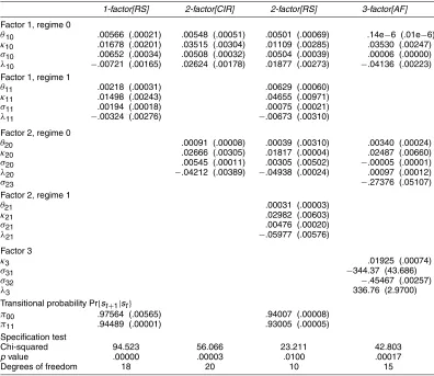
Table 2 gives the main EMM estimation results for four dif-ferent models: one-factor regime-shifting (1-factor[RS]), two-factor square root (2-two-factor[CIR]), two-two-factor regime-shifting (2-factor[RS]), and three-factor affine (3-factor[AF]). Three ad-ditional models (not reported here)—one-factor square root, two-factor Naik and Lee (1997), and three-factor square root— were also estimated, with results similar to those reported by Bansal and Zhou (2002); none of these can replicate the
ex-Table 2. Model Estimation by Efficient Method of Moments
1-factor[RS] 2-factor[CIR] 2-factor[RS] 3-factor[AF]
Factor 1, regime 0
θ10 .00566 (.00021) .00548 (.00051) .00501 (.00069) .14e−6 (.01e−6)
κ10 .01678 (.00201) .03515 (.00304) .01109 (.00285) .03530 (.00247)
σ10 .00652 (.00034) .00508 (.00032) .00504 (.00039) .00006 (.00000)
λ10 −.00721 (.00165) .02624 (.00178) .01877 (.00273) −.04136 (.00223)
Factor 1, regime 1
θ11 .00218 (.00031) .00629 (.00060)
κ11 .01498 (.00243) .04655 (.00971)
σ11 .00194 (.00018) .00075 (.00021)
λ11 −.00324 (.00276) −.00673 (.00310)
Factor 2, regime 0
θ20 .00091 (.00008) .00039 (.00310) .00340 (.00024)
κ20 .02666 (.00305) .01817 (.00004) .02487 (.00660)
σ20 .00545 (.00011) .00305 (.00502) −.00005 (.00001)
λ20 −.04212 (.00389) −.04938 (.00024) .00097 (.00012)
σ23 −.27376 (.05107)
Factor 2, regime 1
θ21 .00031 (.00003)
κ21 .02982 (.00603)
σ21 .00476 (.00020)
λ21 −.05977 (.00576)
Factor 3
κ3 .01925 (.00074)
σ31 −344.37 (43.686)
σ32 −.45467 (.00257)
λ3 336.76 (2.9700)
Transitional probability Pr{st+1|st}
π00 .97564 (.00565) .94007 (.00008)
π11 .94489 (.00001) .93005 (.00005)
Specification test
Chi-squared 94.523 56.066 23.211 42.803
pvalue .00000 .00003 .0100 .00017
Degrees of freedom 18 20 10 15
NOTE: The four term structure models are laid out in Section 2. The 1-factor[RS] or 2-factor[RS] model refers to the regime-shifting specification. The 2-factor[CIR] model is the Cox–Ingersoll–Ross model with two factors. The 3-factor[AF] model is the affine specification mentioned in the text. The simulation size of the EMM is 50,000 for all the four models.
pectation hypothesis puzzle and other data features of interest. The results reported here are for a simulation size of 50,000. The 1-factor[RS] model is rejected with a p value <0. The 2-factor[CIR] model is an improvement, but this specifica-tion is still sharply rejected; the model specificaspecifica-tion test drops to 56.066 with p value < .0003. The best model among all specifications is the 2-factor[RS] model, with apvalue reach-ing 1%. The estimated regime-shiftreach-ing probabilities are both just under .95. All of the parameters of the model are estimated rather accurately. The transition probabilities reported for the 2-factor[RS] specification are comparable to those found by other authors (see Gray 1996; Hamilton 1988; Cai 1994).
The 2-factor[RS] model can be viewed as a three-factor model with the regime-shifting factor being a multiplicative or nonlinear third factor. For a fair comparison of this model, we also estimated a three-factor affine term structure model, (3-factor[AF]), preferred by Dai and Singleton (2000), who found considerable empirical support for this specification us-ing the post-1987 swap yield data. The discrete time counterpart to this affine specification is
X1t+1−X1t=κ1(θ1−X1t)+σ1
Associated with this 3-factor[AF] specification are three mar-ket prices of risk parameters, which, as before, we labelλk,
k=1,2,3. In all, there are 13 parameters to estimate. As ported in Table 2, the 3-factor[AF] specification is sharply re-jected withX2(15)=42.803 and apvalue of .0017. In a more general semiparametric setting, Ghysels and Ng (1998) rejected the affine restrictions on the conditional mean and variance of yields.
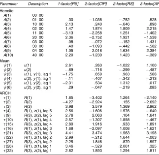
Table 3 reports thet-ratio diagnostics for the 28 moment con-ditions implied by each of the 4 specifications. These 28 scores (moment conditions) should, for a correctly specified model, be close to 0. If the structural model under consideration matches the particular moment under consideration, then at a conventional 5% level of significance, the t-ratio should be smaller than 1.96. The reported t-ratios are not adjusted for parameter estimation, so theset’s are therefore asymptotically slightly downward biased relative to 2.0. They thus must be interpreted with cautious intuition guided by the overall chi-squared diagnostics, which are free of such asymptotic bias. For the 1-factor[RS] model, 17 out of 28 moment tests are re-jected, with fitting of conditional volatility especially bad. The 2-factor[CIR] model has only ninet-ratios higher than 1.96, and adding one more linear factor dramatically improves the fitting of conditional volatility and conditional mean. It is remarkable that our favored 2-factor[RS] model matches well all of the mean, volatility, and polynomial scores, except for the single ARCH(1) score of the 6-month yield that is just over 2.0. The 3-factor[AF] specification is certainly an improvement over the
Table 3. Diagnostic t-Ratios
Parameter Description 1-factor[RS] 2-factor[CIR] 2-factor[RS] 3-factor[AF]
Hermite
NOTE: The SNP score generator is explained in Section 3.2. Thet-ratios are testing whether the fitted sample moments are equal to 0, as predicted by population moments of the SNP density.
one- or two-factor models, but it still has 4 out of 13 ARCH scores and 2 out of 9 Hermite scores that are not well matched. Overall, our preferred 2-factor[RS] specification seems to have the greatest advantage in matching the conditional volatility and covariance (i.e., the ARCH scores) and the non-Gaussian poly-nomials (i.e., the Hermite polynomial parameters) relative to other multifactor CIR or affine specifications.
3.4 Risk Premium Analysis
An important diagnostic is to evaluate whether the dif-ferent model specifications can justify the observed patterns of violations of the expectations hypothesis—in particular, as documented by Fama and Bliss (1987), the predictability of for-ward rates on excess returns. The simple existence of the pre-dictability from forward rate to excess return (R2significantly greater than 0) is easily explained by any dynamic term struc-ture model with time-varying risk premia. However, the greater challenge, as recently popularized by Cochrane and Piazzesi (2002), is to explain the robust tent-shaped pattern of the slope coefficients when multiple forward rates are used as regressors. Another form of the expectation hypothesis violation (not a fo-cus of this article) is the negative slope instead of unity when regressing yield changes on yield spreads (Campbell and Shiller
1991). Bansal and Zhou (2002) provided evidence that the two-factor regime-shifting model is the only one that can replicate this type of expectations hypothesis violation at the shorter ma-turities, whereas all multifactor models fair well at the longer maturities.
Following the same conventions of Cochrane and Piazzesi (2002), we work with log bond prices (i.e.,pkt is the log of the price attof ak yearbond) and geometric (log) yields and re-turns, soy1t = −p1t is the geometric yield on the 1-year bond. Cochrane and Piazzesi (2002) considered the regression of ex-cess returns of bonds on the yields and the forward rates,
exkt+12=βk0+βk1y1t
+
5
i=2
βkifti+ǫtk+12, k=2, . . . ,5, (9)
whereexkt+12=ptk+−121 −pkt−y1t is the excess return on thekyear bond andftk=pkt−1−pkt is the forward rate. Note thatexkt+12
is effectively the return on holding akyear bond for 1 year in excess of the 1-year yield. This excess return data is collected monthly, which leads to the usual overlap in return data.
We first check the robustness of the findings of Cochrane and Piazzesi (2002). As shown in the top panel of Table 4, the
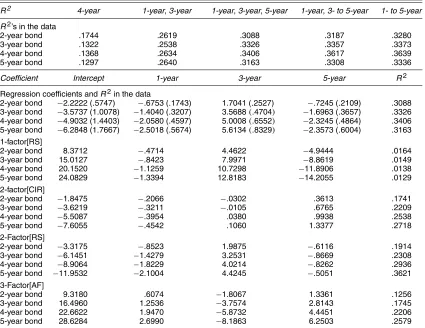
re-Table 4. Predictability of Bond Excess Returns Using Multiple Forward Rates
R2 4-year 1-year,3-year 1-year,3-year,5-year 1-year,3- to 5-year 1- to 5-year
R2’s in the data
2-year bond .1744 .2619 .3088 .3187 .3280
3-year bond .1322 .2538 .3326 .3357 .3373
4-year bond .1368 .2634 .3406 .3617 .3639
5-year bond .1297 .2640 .3163 .3308 .3336
Coefficient Intercept 1-year 3-year 5-year R2
Regression coefficients andR2in the data
2-year bond −2.2222 (.5747) −.6753 (.1743) 1.7041 (.2527) −.7245 (.2109) .3088 3-year bond −3.5737 (1.0078) −1.4040 (.3207) 3.5688(.4704) −1.6963 (.3657) .3326 4-year bond −4.9032 (1.4403) −2.0580 (.4597) 5.0008(.6552) −2.3245 (.4864) .3406 5-year bond −6.2848 (1.7667) −2.5018 (.5674) 5.6134(.8329) −2.3573 (.6004) .3163 1-factor[RS]
2-year bond 8.3712 −.4714 4.4622 −4.9444 .0164
3-year bond 15.0127 −.8423 7.9971 −8.8619 .0149
4-year bond 20.1520 −1.1259 10.7298 −11.8906 .0138
5-year bond 24.0829 −1.3394 12.8183 −14.2055 .0129
2-factor[CIR]
2-year bond −1.8475 −.2066 −.0302 .3613 .1741
3-year bond −3.6219 −.3211 −.0105 .6765 .2209
4-year bond −5.5087 −.3954 .0380 .9938 .2538
5-year bond −7.6055 −.4542 .1060 1.3377 .2718
2-Factor[RS]
2-year bond −3.3175 −.8523 1.9875 −.6116 .1914
3-year bond −6.1451 −1.4279 3.2531 −.8669 .2308
4-year bond −8.9064 −1.8229 4.0214 −.8262 .2936
5-year bond −11.9532 −2.1004 4.4245 −.5051 .3621
3-Factor[AF]
2-year bond 9.3180 .6074 −1.8067 1.3361 .1256
3-year bond 16.4960 1.2536 −3.7574 2.8143 .1745
4-year bond 22.6622 1.9470 −5.8732 4.4451 .2206
5-year bond 28.6284 2.6990 −8.1863 6.2503 .2579
NOTE: The dependent variable in all of the regressions is the 1-year return from holding a bond withnyears to maturity less the yield on a bond with one year to maturity. This annual excess return is tracked monthly. AllR2’s are adjusted for degrees of freedom. The sample size in the data is 451 observations. In the top
panel the predictability regression is run using 1-, 2-, 3-, 4-, and 5-year forward rates as regressors. Because theR2using 1-, 3-, 5-year forward rates is almost
the same as using additional forward rates (see 1-, 3–5, and 1–5 years), we focus on the 1-, 3-, and 5-year projections. Newey–West robust standard errors are reported in parentheses in the “Regression Coefficients andR2in the Data” section for this projection. The results reported for the 1-factor[RS], 2-factor[CIR],
2-factor[RS], and 2-factor[AF] models are based on simulating 50,000 observations from the estimated term structure model and running the same regression as reported in the “Regression Coefficients andR2in the Data” section.
(a) (b)
(c) (d)
(e)
Figure 2. Predictability Regression Coefficients. (a) Observed data; (b) 1-factor[RS] model; (c) 2-factor[RS] model; (d) 2-factor[CIR] model; (e) 3-factor[AF] model ( 2-year bond, 1-year excess return; 3-year bond, 1-year excess return; 4-year bond, 1-year excess return;
5-year bond, 1-year excess return).
gression R2 with five forward rates reaches 36%, which con-firms their findings. An important note is that the difference between using three, four, or five forward rates is negligible, whereas reducing to two or one forward rates dramatically de-creases theR2. This seems to suggest the existence of three la-tent factors, and the use of five regressors creates a near-perfect colinearity problem up to cross-sectional measurement errors
that can mask the singularity. We concentrate on the regres-sions with three forward rates. The estimated coefficients are plotted in Figure 2(a) and the tent-shaped finding of Cochrane and Piazzesi (2002) is quite apparent.
Next, we examine whether any of the dynamic term struc-ture models under consideration can meet the challenge of replicating this unique tent-shaped phenomenon. Using the
timated parameters of the four models, we simulate 50,000 monthly data and run the same regressions of excess bond returns on forward rates. As seen in the lower panel of Ta-ble 4, the 2-factor[RS] model not only achieves the highest predicting R2 (20–36%), but also clearly closely mimics the tent-shaped regression coefficients. On the other hand, the 2-factor[CIR] model produces a skewed and inverted tent shape, and the 3-factor[AF] model produces a inverted tent shape. Both models achieve R2’s around 10–20%. Interest-ingly, even the 1-factor[RS] model can replicate the tent shape to some degree, even though itsR2 is only about 1%. These patterns are quite apparent in Figure 2. These results suggest that the prediction capability of forward rates for excess returns may be explained by two or three linear factors, whereas the tent pattern of regression coefficients appears to be due to the regime-shifting nature of the yield curve.
The analysis of Duffee (2002) and Dai and Singleton (2002) suggest that allowing more flexible specification of the risk pre-mium parameters for the conditional Gaussian factor model can dramatically improve its ability to match the predictability of excess returns. To explore this argument, we have also esti-mated the “preferred essentially affineA0(3)model” discussed by Duffee (2002) with three Gaussian factors and eight market-price-of-risk parameters (we call it the 3-factor[EA] model). The chi-squared test of overall specification is 29.278 with 9 de-grees of freedom and apvalue of .0006; hence the model is not supported by the data. The estimation result suggests that the 3-factor[EA] model overshoots the excess returns predictabil-ity, theR2range from 26% to 65% vis-a-vis 30% observed in the data. More importantly, it cannot reproduce the tent shape of the predictability regression coefficients. Further, its perfor-mance for cross-sectional pricing error is somewhat worse than that of the three-factor affine model. Our diagnostics for this model specification reveal that the implied conditional volatil-ity and conditional correlations of yields do not match those in the data. Given this result, for brevity we do not present very detailed evidence on this specification.
3.5 Regime Indicator, Risk Premium, and the Business Cycle
We now explore the cross-sectional implications of the term structure models over the maturities that are not used in the model estimation. We also look at the association between the bond market implied regimes and the real business cycle. For the 2-factor[CIR] and 3-factor[AF] models, a standard method is used to calculate the pricing errors. Because the yield curve solution is linear in the factors, we first invert from two or three basis yields to get the latent factors and then use the lin-ear pricing solution to calculate the nonbasis yields. For the 1-factor[RS] and 2-factor[RS] models, the presumption that agents in the economy know the current regime implies a strat-egy to recover the regimes. Specifically, dates are classified into regimes according to which of the two yield curves produces the smallest pricing error. Under the null of correct specifica-tion, the pricing error should be 0 given the true regime and the population parameter values (for more details, see Bansal and Zhou 2002).
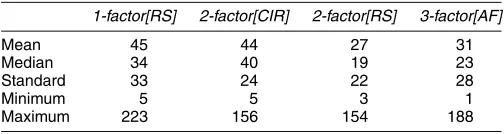
Table 5. Average Absolute Pricing Error (basis points)
1-factor[RS] 2-factor[CIR] 2-factor[RS] 3-factor[AF]
Mean 45 44 27 31
Median 34 40 19 23
Standard 33 24 22 28
Minimum 5 5 3 1
Maximum 223 156 154 188
NOTE: There are eight maturities (1-, 3-, and 6-month; and 1-, 2-, 3-, 4-, and 5-year) for each of 451 dates. The absolute pricing errors over 7 points for the 1-factor[RS] model; over 6 points for the 2-factor[CIR] model; over 6 points for the 2-factor[RS] model and over 5 points for the 3-factor[AF] model. The summary statistics of the absolute pricing errors are calculated over the 451 dates for each of the 4 models.
Table 5 reports the time-series average of pricing errors 1/TT
t=1PEs(t)or other statistics from the cross-sectional av-erage PEs(t)=1/NNn=1| ˆYs(t,n)−Ys(t,n)|, whereYˆs(t,n)is the calculated yield andYs(t,n)is the observed yield for ma-turity n at time t (where the current states is inferred from minimizing the pricing errors of the two yield curves, as men-tioned earlier). It is clear from the sample statistics that the 2-factor[RS] model has the smallest average pricing error and also the smallest standard deviation in the pricing error. The maximal pricing error associated with the 2-factor[RS] specifi-cation is also the smallest. Further, on average the pricing er-ror is only about 27 basis points for the annualized percentage yields. The 3-factor[AF] specifications have average pricing er-rors of 31 basis points, which in an absolute sense is also quite small. The 1-Factor[RS] and 2-factor[CIR] models achieve sim-ilar pricing results as 44 to 45 basis points.
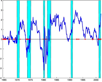
It has been well recognized that the slope of the yield curve (i.e., spread) has the ability to predict future real GDP growth; in particular, negative spreads tend to predict a recession (see, e.g., Harvey 1988; Estrella and Hardouvelis 1991). Figure 3 recreates this linkage between the monthly yield spread, our regime indicator for regime 0 (our low regime), and the Na-tional Bureau of Economic Research (NBER) business cycles recession indicator. Most of the time, it seems that the economy is in regime 1. The total number of regime switches recovered from the sample period is 44. The regime relates to the NBER business cycles. Our low regime (regime 0) obtains during or before recessions in the economy. In the data, the correlation between NBER business cycle indicator and the yield spread (5-year yield minus 6-month yield) is 15%. In general, the yield curve becomes inverted (or flat) several months before the eco-nomic growth becomes negative (or depressed). Our regime in-dicator is mostly 0, as Figure 3 shows, when the yield curve becomes inverted (or flat). The correlation between the model-based regime indicator and the yield spread (5-year yield minus 6-month yield) is 24%; that is, our high regime (regime 1) co-incides with a high yield spread and our low regime (regime 0) largely coincides with a low yield spread. Therefore, as reported by Bansal and Zhou (2002), the regime indicator has the power to predict recessions. The correlation between the NBER busi-ness cycle (NBER recession as regime 0 and NBER boom as regime 1) and our regime indicator is .1117. In the context of modeling the short interest rate, Ang and Bekaert (2002) also documented the links between regime shifts and business cy-cles.
Fama and Bliss (1987) attributed the time-varying risk pre-mium in bonds to the business cycle. In particular, their argu-ment is that the bond excess return is high when the economy
Figure 3. Yield Spread, Regime Indicator, and Business Cycle. The thick line is the 5-year yield minus the 6-month yield (yield spread), the shaded area is the NBER recession period, and the star is the indicator of our low regime (regime 0) from our preferred 2-factor[RS] model. The high regime (regime 1) corresponds to all dates without the star.
is in recessions and low when it is in expansions. Figure 4(a) shows that our regime 0 and negative ex-post excess returns bear close relation; the correlation between our regime indica-tor and ex-post bond excess returns is 21%. That is, our high regime (regime 1) tends to coincide with high ex-post returns. We also explore how the expected excess returns relate to the regimes. Figure 4(b) plots the fitted expected return in the data based on the excess return forward rate projection discussed earlier. The correlation in the data between our regime indica-tor and the expected excess return is 32%; that is, high risk pre-mia and the high regime (regime 1) tend to go together. In this sense our regimes can also be thought of as ranking on high and low risk premia on bonds. Figure 4(c) plots the reprojected ex-pected excess returns for bonds from our preferred 2-factor[RS] model. The reprojected expected excess return for this model duplicates the expected excess return patterns observed in the data. Further, the reprojected expected excess return has a cor-relation of 37% with our regime indicator. The overall evidence indicates that our regime indicator tracks the time-varying risk premium on the bond market. As discussed earlier, none of the other models can replicate the Cochrane and Piazzesi (2002) predictability regressions; consequently, none also cannot ac-count for the expected risk premium dynamics plotted in Fig-ure 4(b).
3.6 The Reprojected Conditional Volatility and Correlation
As a final diagnostic, we assess the ability if the various mod-els to match the shape and track the conditional distribution and covariance characteristics of the data. Following Gallant
and Tauchen (1998), we compute the reprojected conditional density of the two basis yields. Given the estimated null model and the simulated output for yields, the reprojected conditional density is obtained by reestimating the parameters of the SNP density. Moments of interest, such as the conditional variances and correlations implied by the model specification, can then be computed. These conditional moments are simply functions of the conditioning information used to estimate the reprojected density. Given the conditioning information, the implications of a given null model for any conditional moment of interest can be evaluated on the observed data and compared to the condi-tional moment implied by the unrestricted SNP density.
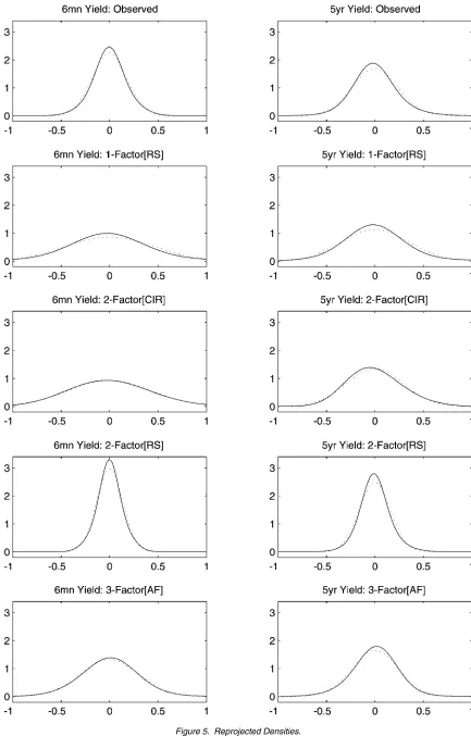
Figure 5 plots the reprojected conditional density (evaluated at the sample mean), for the different models under consid-eration. The unrestricted 6-month yield SNP density has high peak and narrow shoulders, and the unrestricted density for the 5-year yield is skewed to the left and moderately peaked. The reprojected densities for the 3-factor[AF] model do cap-ture the peakedness of the 5-year yield but miss the peak of the 6-month yield and the skew of the 5-year yield. On the other hand, the reprojected densities for the 1-factor[RS] and 2-factor[CIR] models capture the skewness of the 5-year yield somewhat but largely miss the peak of both yields. The 2-factor[RS] regime-shifting model has greater success in cap-turing the left skew of the 5-year yield and the peak of both yields.
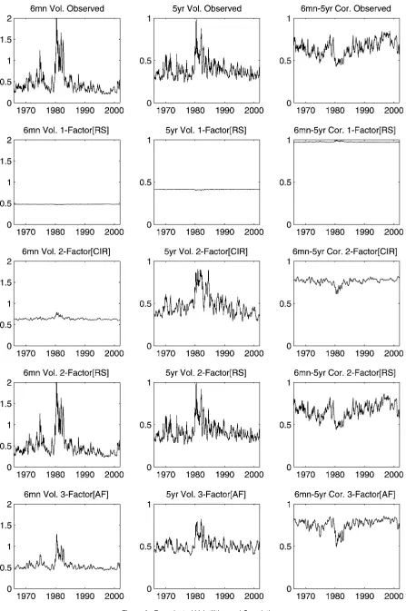
Figure 6 displays the conditional volatility and cross-correlation for the various model specifications as implied by the reprojected densities. Note that in the data, the dynamics of the conditional variance of the 6-month yield is quite differ-ent from that of the 5-year yield. The range for the conditional
(a)
(b)
(c)
Figure 4. Excess Return, Regime Indicator, and the Business Cycle. The shaded area is the NBER recession period, and the star is the indicator of the low regime (regime 0) from our preferred regime-shifting term structure model. The thick line represent the annual ex-post excess return (a), the expected excess return based on projecting future ex-post excess returns on three forward rates (b), and the reprojected expected excess return from our 2-factor[RS] model (c). All ex-post and expected excess returns are averages (across bonds) using the 2- to 5-year bonds.
volatility for the 6-month yield rate is much larger than for the 5-year yield—the high end being almost three times the lowest for the 6-month yield and two times the lowest for the 5-year yield. The short yield volatility is more persistent, whereas the long yield volatility seems more choppy. The 1-factor[RS] model does not reflect any time variations of short and long rate volatilities, although the levels of volatility are matched. The 2-factor[CIR] model has difficulty in matching the short rate volatility and does somewhat better in matching the volatil-ity of the 5-year yield. The 2-factor[RS] model is capable of duplicating the projected volatility of the short rate extremely well and that of the long yield volatility almost completely. The 3-factor[AF] model seems to capture the volatility of the short rate much better than the 2-factor[CIR] model; however, its ca-pability to mimic the long rate volatility is diminished relative to the 2-factor[CIR] model.
The rightmost plots of Figure 6 provide evidence regard-ing the conditional correlation between the 6-month and 5-year yields. The 2-factor[RS] model succeeds in capturing the wide
range of the correlation observed across these yields. The cor-relation varies from 40% to 80%. Note that although the condi-tional volatility increases during the volatile period of the early 1980s, the conditional correlation decreases, suggesting that the volatilities of the two yields rise more rapidly relative to the conditional covariance. The 1-factor[RS] model, with only one linear factor, not surprisingly presents a nearly constant correla-tion very close to unity. The 2-factor[CIR] and the 3-factor[AF] specifications have difficulty capturing the conditional covari-ance. However, the 3-factor[AF] specification seems doing a considerably better job of capturing the conditional covariance relative to the 2-factor[CIR] specification. The 2-factor[RS] model comes quite close to capturing virtually all of the ob-served dynamics of the conditional correlation between these yields. The main message of this evidence is that our preferred regime-shifting term structure model is quite successful in cap-turing the conditional volatility and cross-correlation dynamics of yields. In addition, it captures the size and nature of the pre-dictability of bond returns.
Figure 5. Reprojected Densities.
Figure 6. Reprojected Volatilities and Correlations.
4. CONCLUDING REMARKS
Business cycle movements between economic expansions and recessions affect macroeconomic variables, financial mar-kets, and, in particular, the term structure of interest rates. In this article we have incorporated the well-documented feature of regime shifts as given by Hamilton (1988) into the standard term structure model such as that of Cox et al. (1985). We have uncovered additional important new evidence on the empirical success of regime-switching models beyond that reported by Bansal and Zhou (2002).
The empirical work was conducted on nominal U.S. treasury bill and bond yields from 1964 to 2001. For estimation and specification tests of the various models, we used the EMM esti-mation technique developed by Bansal et al. (1995) and Gallant and Tauchen (1996). A two-factor regime-shifting model is the only specification that fits the data according to the usual chi-squared test of the restrictions; other models, including the mul-tifactor CIR and affine, are rejected. Furthermore, the preferred two-factor regime-shifting model matches the semiparametric moments with acceptablet-ratio diagnostics. In terms of cross-sectional implications, the preferred model achieves the small-est pricing error among all of the specifications considered.
Regime shifting and the risk premium for holding bonds ap-pear to be closely connected. We have shown that the main channel that the regime-shifting model accommodates is a time-varying “beta” with respect to risk factors. Our empirical evidence indicates that of the considered models, only the regime-shifting model can account for the size of the pre-dictability (i.e., highR2’s) and the tent-shaped structure of re-gression coefficients in the generalized expectations hypothesis regressions of excess bond returns on forward rates (Cochrane and Piazzesi 2002). It is also able to account for the condi-tional volatility and condicondi-tional cross-correlation across yields. We find that there is an intimate link between business cycles, the slope of the yield curve, expected excess return of bonds, and the regimes extracted from our term structure model.
ACKNOWLEDGMENTS
The authors thank John Cochrane, Ron Gallant, Eric Ghysels, Monika Piazzesi, and the seminar participants at the NSF Time Series Conference and the Federal Reserve Board for helpful comments and suggestions. The views expressed in this arti-cle reflect those of the authors and do not represent those of the Board of Governors of the Federal Reserve System or other members of its staff.
[Received January 2003. Revised December 2003.]
REFERENCES
Ahn, D.-H., Dittmar, R. F., and Gallant, A. R. (2002), “Quadratic Term Structure Models: Theory and Evidence,”Review of Financial Studies, 15, 243–288.
Ang, A., and Bekaert, G. (2002), “Regime Switches in Interest Rates,”Journal of Business & Economic Statistics, 20, 163–182.
Bansal, R., Gallant, A. R., Hussey, R., and Tauchen, G. (1995), “Nonparametric Estimation of Structural Models for High-Frequency Currency Market Data,”
Journal of Econometrics, 66, 251–287.
Bansal, R., and Zhou, H. (2002), “Term Structure of Interest Rates With Regime Shifts,”Journal of Finance, 57, 1997–2043.
Cai, J. (1994), “A Markov Model of Switching-Regime ARCH,”Journal of Business & Economic Statistics, 12, 309–316.
Campbell, J. Y., and Shiller, R. J. (1991), “Yield Spreads and Interest Rate Movements: A Bird’s Eye View,”Review of Economic Studies, 58, 495–514. Chernov, M., Gallant, A. R., Ghysels, E., and Tauchen, G. (2003), “Alternative Models for Stock Price Dynamics,”Journal of Econometrics, 116, 225–257. Cochrane, J. H., and Piazzesi, M. (2002), “Bond Risk Premia,” working paper,
University of Chicago and University of California Los Angeles.
Cox, J. C., Ingersoll, J. E., and Ross, S. A. (1985), “A Theory of the Term Structure of Interest Rates,”Econometrica, 53, 385–407.
Dai, Q., and Singleton, K. J. (2000), “Specification Analysis of Affine Term Structure Models,”Journal of Finance, 55, 1943–1978.
(2002), “Expectation Puzzles, Time-Varying Risk Premia, and Affine Models of the Term Structure,” Journal of Financial Economics, 63, 415–441.
Dai, Q., Singleton, K. J., and Yang, W. (2003), “Regime Shifts in a Dynamic Term Structure Model of the U.S. Treasury Yields,” working paper, Stern New York University and GSB Stanford University.
Duffee, G. (2002), “Term Premia and Interest Rate Forecasts in Affine Models,”
Journal of Finance, 57, 405–443.
Engle, R. F., and González-Rivera, G. (1991), “Semiparametric ARCH Mod-els,”Journal of Business & Economic Statistics, 9, 345–359.
Estrella, A., and Hardouvelis, G. A. (1991), “The Term Structure as a Predictor of Real Economic Activity,”Journal of Finance, 46, 555–576.
Evans, M. D. D. (2003), “Real Risk, Inflation Risk, and the Term Structure,”
The Economic Journal, 113, 345–389.
Fama, E. F., and Bliss, R. T. (1987), “The Information in Long-Maturity For-ward Rates,”American Economic Review, 77, 680–692.
Gallant, A. R., and Tauchen, G. (1996), “Which Moment to Match?” Econo-metric Theory, 12, 657–681.
(1998), “Reprojecting Partially Observed Systems With Application to Interest Rate Diffusions,”Journal of the American Statistical Association, 93, 10–24.
(1999), “The Relative Efficiency of Method of Moments Estimators,”
Journal of Econometrics, 92, 149–172.
Garcia, R. (1998), “Asymptotic Null Distribution of the Likelihood Ratio Test in Markov Switching Models,”International Economic Review, 39, 763–788. Ghysels, E., and Ng, S. (1998), “A Semiparametric Factor Model of Interest
Rates and Tests of the Affine Term Structure,”Review of Economics and Statistics, 80, 535–548.
Gray, S. F. (1996), “Modeling the Conditional Distribution of Interest Rates as a Regime-Switching Process,”Journal of Financial Economics, 42, 27–62. Hamilton, J. D. (1988), “Rational Expectations Econometric Analysis of
Changes in Regimes: An Investigation of the Term Structure of Interest Rates,”Journal of Economic Dynamics and Control, 12, 385–423.
(1989), “A New Approach to the Economic Analysis of Nonstationary Time Series and the Business Cycle,”Econometrica, 57, 357–384. Hansen, B. E. (1992), “The Likelihood Ratio Test Under Non-Standard
Con-ditions: Testing the Markov Switching Model of GNP,”Journal of Applied Econometrics, 7, s61–s82.
Hansen, L. P., and Jagannathan, R. (1997), “Assessing Specification Errors in Stochastic Discount Factor Models,”Journal of Finance, 52, 557–590. Harvey, C. R. (1988), “The Real Term Structure and Consumption Growth,”
Journal of Financial Economics, 22, 305–333.
Naik, V., and Lee, M. H. (1997), “Yield Curve Dynamics With Discrete Shifts in Economic Regimes: Theory and Estimation,” working paper, University of British Columbia, Faculty of Commerce.
Roberds, W., and Whiteman, C. H. (1999), “Endogenous Term Premia and Anomalies in the Term Structure of Interest Rates: Explaining the Pre-dictability Smile,”Journal of Monetary Economics, 44, 555–580.
![Figure 2. Predictability Regression Coefficients. (a) Observed data; (b) 1-factor[RS] model; (c) 2-factor[RS] model; (d) 2-factor[CIR] model;](https://thumb-ap.123doks.com/thumbv2/123dok/1145540.764948/9.612.118.512.42.596/figure-predictability-regression-coefcients-observed-factor-factor-factor.webp)