Full Terms & Conditions of access and use can be found at
http://www.tandfonline.com/action/journalInformation?journalCode=ubes20
Download by: [Universitas Maritim Raja Ali Haji] Date: 11 January 2016, At: 23:19
Journal of Business & Economic Statistics
ISSN: 0735-0015 (Print) 1537-2707 (Online) Journal homepage: http://www.tandfonline.com/loi/ubes20
Bayesian Time-Varying Quantile Forecasting for
Value-at-Risk in Financial Markets
Richard H. Gerlach, Cathy W. S. Chen & Nancy Y. C. Chan
To cite this article: Richard H. Gerlach, Cathy W. S. Chen & Nancy Y. C. Chan (2011) Bayesian Time-Varying Quantile Forecasting for Value-at-Risk in Financial Markets, Journal of Business & Economic Statistics, 29:4, 481-492, DOI: 10.1198/jbes.2010.08203
To link to this article: http://dx.doi.org/10.1198/jbes.2010.08203
Published online: 24 Jan 2012.
Submit your article to this journal
Article views: 675
View related articles
Bayesian Time-Varying Quantile Forecasting for
Value-at-Risk in Financial Markets
Richard H. G
ERLACHDiscipline of Operations Management and Econometrics, University of Sydney, NSW 2006, Australia (richard.gerlach@sydney.edu.au)
Cathy W. S. C
HENDepartment of Statistics, Feng Chia University, 407, Taiwan (chenws@fcu.edu.tw)
Nancy Y. C. C
HANDepartment of Statistics, Feng Chia University, 407, Taiwan (ycchan@fcu.edu.tw)
Recently, advances in time-varying quantile modeling have proven effective in financial Value-at-Risk forecasting. Some well-known dynamic conditional autoregressive quantile models are generalized to a fully nonlinear family. The Bayesian solution to the general quantile regression problem, via the Skewed-Laplace distribution, is adapted and designed for parameter estimation in this model family via an adaptive Markov chain Monte Carlo sampling scheme. A simulation study illustrates favorable precision in esti-mation, compared to the standard numerical optimization method. The proposed model family is clearly favored in an empirical study of 10 major stock markets. The results that show the proposed model is more accurate at Value-at-Risk forecasting over a two-year period, when compared to a range of existing alternative models and methods.
KEY WORDS: Asymmetric; CAViaR model; GARCH; Regression quantile; Skewed-Laplace distribu-tion.
1. INTRODUCTION
Value-at-Risk (VaR) is the benchmark for risk measure-ment and subsequent capital allocation for financial institutions worldwide, as chosen by the Basel Committee on Banking Su-pervision (see Basel II: http:// www.bis.org/ publ/ bcbsca.htm). VaR is a one-to-one function of a quantile, over a given time in-terval, of an asset portfolio’s conditional return distribution (see Jorion1996). Many competing models/methods have been used in the literature to estimate and forecast quantiles, and hence VaR (see Kuester, Mittnik, and Paolella2006for a review). We focus on the conditional autoregressive VaR (CAViaR) models proposed by Engle and Manganelli (2004), to estimate quan-tiles (VaR) directly, and expand the existing CAViaR models into a fully nonlinear family of dynamic models, in the spirit of threshold GARCH modeling (see Zakoian1994and Brooks
2001). Such models capture a range of nonlinear and asym-metric behavior, including the well-known leverage effect, or volatility asymmetry, discovered by Black (1976).
Manganelli and Engle (2004) find that the classical numer-ical optimization procedure for quantile models of Koenker and Bassett (1978) is inefficient and problematic at very low quantiles, and presumably at low sample sizes as well, for CAViaR models. This article develops a Bayesian estimator for the proposed nonlinear CAViaR model family, adapted from the MCMC sampling scheme of Chen and So (2006). This MCMC estimator takes advantage of the gains in efficiency that numer-ical integration, for estimating the posterior mean, can display over standard numerical differentiation based optimisation, for example, in Engle and Manganelli (2004), especially in mod-els with many parameters. The MCMC scheme is adaptive, ex-panding the MCMC methods for general quantile regression
models in Yu and Moyeed (2001), Tsionas (2003), and Geraci and Bottai (2007).
Parametric GARCH-type models (see, e.g., Engle1982and Bollerslev 1986), with specified error distributions, are also well suited to quantile forecasting and are often used as bench-marks in VaR studies (e.g., Kuester, Mittnik, and Paolella
2006). However, some financial institutions employ sample re-turn quantiles, called historical simulation (HS), for nonpara-metric estimation of VaR. Manganelli and Engle (2004) find that the basic CAViaR model outperforms standard GARCH and HS approaches for forecasting VaR from simulated data, especially for fat-tailed error processes. We show that this result also holds for some real market return data, at the 1% quantile level. Giacomini and Komunjer (2005) develop an encompass-ing test for forecast models and find that a CAViaR model is most useful at the 1% quantile level, but that a simple GARCH model with Gaussian errors outperforms the CAViaR model at the 5% level, for the U.S. S&P500 return data from 1985– 2001. We extend these results in this article across 10 inter-national market indices, finding that this conclusion general-izes across these markets, in a more recent time period. Fur-ther, Geweke and Keane (2007) propose a smoothly mixing re-gression approach to semiparametrically and flexibly estimate predictive densities, a method that can capture some types of heteroscedasticity. This approach outperforms GARCH models for the U.S. S&P500 index from 1995–1999. We consider all the above-mentioned VaR forecasting approaches in this arti-cle.
© 2011American Statistical Association Journal of Business & Economic Statistics October 2011, Vol. 29, No. 4 DOI:10.1198/jbes.2010.08203
481
The proposed full model and MCMC methods are examined first through a simulation study, and second through application to various financial market stock indices in a study of VaR fore-casting. The simulation study illustrates favorable estimation performance, in terms of precision and efficiency, compared with numerically optimizing the usual quantile criterion func-tion. The empirical study illustrates that CAViaR models per-form favorably compared to RiskMetrics and general GARCH estimators, for VaR forecasting, during the period 2005–2007, especially at the 1% quantile level; while simpler models, in-cluding GARCH and RiskMetrics do comparably well at the 5% quantile level.
The article is organized as follows: Section2discusses dy-namic quantile estimation; Section 3 introduces the proposed family of dynamic autoregressive quantile models; Section 4
presents the MCMC methods employed; Sections5and6, re-spectively, present the simulation and empirical studies; and some concluding remarks are given in Section7.
2. DYNAMIC QUANTILE AND VALUE–AT–RISK
This section discusses the general dynamic quantile problem and the relation to the Skewed Laplace (SL) distribution. The general dynamic quantile model may be written
yt=ft(β,xt−1)+ut, (1)
whereyt is the observation at timet;xt−1are the explanatory variables;β are unknown parameters and ut is an error term.
The functionft(·)defines the dynamic link betweenytandxt−1 and is usually linear inβandx, an aspect that is extended here. The conditionalαlevel quantile is then
qα(yt|β,xt−1)=ft(βα,xt−1),
Yu and Moyeed (2001) and Tsionas (2003) illustrate the link between the solution to the quantile estimation problem and the likelihood for the SL distribution, as follows. The SL location-scale family, denoted SL(μ, τ, α), has density function
pα(u)=
Since (2) is contained in the exponent of the likelihood, the maximum likelihood estimate forβis equivalent to the quantile estimator in (2).
It is important to emphasize that, though we treat (4) as a like-lihood function, the assumption thaty follows an SL(μ, τ, α) distribution is not used to parametrically estimate VaR. In prac-tice, the parameterαis fixed and known during parameter esti-mation and only that single quantile of the distribution ofytis
estimated. Equation (4) is only employed as it leads to (maxi-mum likelihood) estimation that is mathematically equivalent to (2). Use of (4) as a likelihood function, then allows a Bayesian approach to consider powerful computational estimation meth-ods, such as adaptive MCMC algorithms, that employ numer-ical integration (which can be made arbitrarily accurate), in-stead of numerical optimization. Authors such as Yu and Moy-eed (2001) and Tsionas (2003) have illustrated that accurate Bayesian estimation and inference is achieved under this ap-proach. We further investigate and add to these findings for dy-namic nonlinear quantile models.
2.2 Value-at-Risk
The Basel Capital Accord, originally signed by the Group of Ten countries in 1988, requires Authorized Deposit-taking In-stitutions to hold sufficient capital to provide a cushion against unexpected losses. VaR forecasts the minimum expected loss over a given time interval, at a given confidence levelα(Jorion
1996). That is,
α=Pr(yt<−VaRt|y1,t−1).
VaR is thus proportional to a quantile in the conditional one-step-ahead forecast distribution.
As in Manganelli and Engle (2004) VaR estimation methods can be classified as parametric, with a full distributional and model form specified; nonparametric, with minimal or no dis-tributional or model assumptions; and semiparametric, where some assumptions are made, either about the error distribution, or the model dynamics, but not both (e.g., quantile regression and CAViaR models). Monte Carlo (MC) simulation methods are commonly used in all three categories.
A popular parametric method for VaR estimation is RiskMet-rics (RMetRiskMet-rics), proposed by J. P. Morgan in1996, where an IGARCH(1,1)process, with no mean equation, is employed. For expositional purposes, the standard GARCH(1,1)model is
yt=μ+at; at=σtǫt, ǫt and is thus nonstationary in volatility. Standard GARCH the-ory (e.g., see Tsay2005) allows closed form solutions to the one-step-ahead quantiles ofyt|y1,t−1, given the parameter
val-ues and based on parametric errors. From here on, the stan-dard GARCH(1,1)with Gaussian errors is labeled GARCH-n, while the GARCH(1,1)with standardized Student-t errors is denoted GARCH-t.
2.3 CAViaR Models for VaR
Engle and Manganelli (2004) propose various dynamic quan-tile functionsf(·), which they called CAViaR models. We ini-tially discuss three of their specifications:
IndirectGARCH(1,1)(IG):
ft(β)= [β1+β2ft2−1(β)+β3y2t−1]1/2. (5) This equation is exactly equivalent to the dynamic quantile function for a GARCH(1,1)model with an iid symmetric error distribution and meanμ=0. The model thus allows efficient estimation for GARCH(1,1)quantiles with unspecified error distribution. This is an advantage: GARCH models are typi-cally estimated under a parametric error distribution. However, it is well known that standard GARCH models tend to overre-act to large return shocks (since they are squared). As such we prefer the absolute value model types below:
Symmetric Absolute Value(SAV):
ft(β)=β1+β2ft−1(β)+β3|yt−1|. (6) The quantile again responds symmetrically to the lagged return
yt−1. This equation is equivalent to the quantile function for a
standard deviation GARCH model (see, e.g., Zakoian 1994), where
σt=γ1+γ2σt−1+γ2|at−1|.
The two CAViaR models SAV and IG have symmetric re-sponses to positive and negative observations. To account for fi-nancial market asymmetry, via the leverage effect (Black1976), the SAV model is extended in Engle and Manganelli (2004) to
Asymmetric Slope(AS): where the dynamic quantile function can respond differently to positive and negative responses. Such a threshold non-linear model is similar in spirit to the GJR-GARCH model (Glosten, Jagannathan, and Runkle1993) or EGARCH (Nelson
1991), where asymmetry is modeled by adding one parameter only, and hence the types of asymmetry captured are limited. Again the AS model corresponds to a standard deviation GJR-GARCH model with meanμ=0 where
σt=δ1+δ2σt−1+δ3I(at−1>0)|at−1| +δ4I(at−1<0)|at−1|. We expand these CAViaR models in Section 3 to capture more flexible asymmetric and nonlinear responses, via more general threshold nonlinear forms.
3. PROPOSED NONLINEAR DYNAMIC QUANTILE FAMILY
A popular model for explaining asymmetry in the mean is the threshold autoregressive (TAR) model of Tong (1978,1983). As a natural extension of this model, Li and Li (1996) and Brooks (2001) modeled mean and volatility asymmetry together, ex-panding the first generation ARCH and GARCH models to be fully threshold nonlinear. In the same spirit, it is natural to ex-tend the SAV and AS (CAViaR) models to the following thresh-old CAViaR model:
Here z is an observed threshold variable which could be ex-ogenous, or self-exciting, that is,zt=yt andris the threshold
value, typically set asr=0, or estimated, though empirically many estimates in the literature are not significant from zero; as such we fixr=0, which also makes the T-CAViaR a direct extension of the AS-CAViaR model in (7). We consider both exogenous and self-exciting threshold variables in this article. The exogenous threshold is the return on the U.S. S&P500 in-dex and the model using that threshold is denoted as TCAVx. The self-exciting model is denoted TCAV.
Here each parameter in the dynamic quantile function can respond differently to positive and negative responses. We call this the T-CAViaR family since it includes the SAV (r= ∞) and AS (r=0, β4=β1 andβ5=β2) CAViaR models as special cases. Once again, this model is the semiparametric equivalent of the standard deviation T-GARCH model with meanμ=0
σt=
δ
1+δ2σt−1+δ3|at−1|, zt−1≤0 δ4+δ5σt−1+δ6|at−1|, zt−1>0.
(9)
We choose to focus on this absolute value CAViaR model-type. However, a corresponding T-CAViaR-IG model could be spec-ified as
We limit focus in this article to the T-CAViaR model fam-ily (8). These models are nonparametric in their error specifi-cations, but simply extend the existing forms for the dynamic function f(·)to be fully threshold nonlinear: that is, they are semiparametric. Yu, Li, and Jin (2010) extend CAViaR us-ing two approaches, namely the threshold and mixture type indirect-VaR models.
Dynamic models typically have constraints or restrictions on the parameters for stationarity (or positivity of dynamic vari-ances). However, such restrictions are difficult to locate or de-rive for CAViaR models, and we choose not to set any in this article, as in Engle and Manganelli (2004).
4. BAYESIAN METHODS
Bayesian methods generally require the specification of a likelihood function and a prior distribution. The likelihood function for the T-CAViaR is completely specified by (4) and (8). We now specify the prior distribution.
4.1 Prior and Posterior Densities
We choose the prior to be uninformative over the possible region for the regression-type parametersβ. The joint prior is thus
π(β)∝1,
which is equivalent to a flat prior onβover the real line, in six dimensions. Yu and Moyeed (2001) showed that the posterior
inβ is proper, under this improper prior, for general quantile
which is in the form of an inverse gamma density in τ. Since estimation ofτ is not relevant in VaR forecasting, this parame-ter is integrated out of (11), to obtain the marginal posterior for
β|y:
using the fact that the inverse gamma density integrates to 1. This posterior is not in a form permitting direct inference on
β. We thus turn to computational methods for estimation and inference.
4.2 Adaptive MCMC Sampling Using Metropolis Methods
Sampling fromp(β|y)directly is not possible given the non-standard form, so instead a dependent (Markov chain) Monte Carlo sample is obtained from (12) via the Metropolis and Metropolis–Hastings (MH) (Metropolis et al. 1953; Hastings
1970) algorithms. To speed convergence and to allow desirable mixing properties in the chain, an adaptive MCMC algorithm forβ|yis employed combining a random walk Metropolis (RW-M) and an independent kernel (IK-) MH algorithm.
We modify the adaptive sampling scheme of Chen and So (2006), who used Gaussian proposal densities. Such a proposal can get “stuck” in local modes and take a large number of it-erates to move out of that area of the posterior. To improve on this aspect, for the burn-in period iterations, a Student-t pro-posal distribution, with low degrees of freedom (e.g., df=5), is employed in a RW-M algorithm. The scale matrix, which can be chosen as diagonal with positive values, is subsequently tuned to achieve optimal acceptance rates of between 20% and 50%, based on recommendations in Gelman, Roberts, and Gilks (1996) and Chen and So (2006). After the burn-in period, the sample mean vector and sample variance–covariance matrix are formed using theseMiterates ofβ. These are subsequently em-ployed in the sampling period (iterations M+1 toN) as the mean and scale matrix for another Student-tproposal distribu-tion in an IK-MH algorithm.
This adaptive proposal updating procedure should speed mixing in the posterior distribution, over that for the simple RW-M method, as long as the burn-in period has “covered” the posterior distribution. The Student-t proposals employed here will further assist in achieving coverage and mixing, over the Gaussian, for both the burn-in and sampling periods, by low-ering the probability of getting stuck in local modes for long
periods and allowing for occasional large jumps around the pos-terior space. We extensively examined trace plots and autocor-relation function (ACF) plots, from multiple runs of the MCMC sampler, from differing starting points, for each element ofβ, so as to confirm convergence and to infer adequate coverage. We also employed Gelman’s ‘R’ statistic (see Gelman et al.
2005, p. 296), which assesses speed of mixing and efficiency of convergence. The values obtained for real and simulated data are typically very close to 1, and almost always below 1.05, implying fast mixing and good convergence properties, for all parameters. Observed MH acceptance rates for this scheme are usually from 15%–40%.
5. SIMULATION STUDY
A simulation study is performed to study the comparative performance of the proposed MCMC method and the classical quantile estimator (2), in terms of parameter and quantile esti-mation and forecasting. The aim is to partially illustrate simi-lar lack of bias for these two methods, while highlighting the increased precision of the MCMC estimator. The results pre-sented focus on the full T-CAViaR model only; results employ-ing the AS and SAV models are available from the authors on request: they are very similar to those presented here.
A specific choice of parametric error distribution is needed here. We choose the equivalent, to the full T-CAViaR model, standard deviation T-GARCH in (9). Samples of sizen=2000 were simulated from this model, with Student-terrors, specified as
6 represents the standardized Student-tdistribution with ν=6. The true one-step-aheadαquantile is thenqα(yt+1|β)=
6 is the inverse Student-tcdf. 400 datasets were simulated. The full T-CAViaR model is fit to each, once using the MCMC method in Section4 and secondly using the classical estimator, employing the ‘fmin-search’ routine in Matlab software, to numerically minimize (2). The Matlab code employed is adapted, and updated for the full T-CAViaR model, from freely available code writ-ten by Simone Manganelli; downloadable from http:// www. simonemanganelli.org/ Simone/ Research.html. The MCMC sample size isN=40,000, with a burn-in ofM=15,000, it-erations. Initial values were randomly set inside(0,1)for each parameter. For the classical estimator, a grid of starting values were chosen for each parameter (from[−1,1]), then parame-ter estimates, starting from each set of grid values, were found; the global minimum value of (2) gave the final classical esti-mates. VaR estimates in-sample, as well as a one-step-ahead forecast for VaR at time n+1=2001 were also calculated. Following Basel II risk management guidelines, quantile levels ofα=0.01,0.05 were considered.
Estimation results are summarized in Table 1. The corre-sponding parameters of the T-CAViaR model are: β1(α) =
Table 1. Summary statistics for the two estimators of the T-CAViaR model using data simulated from a T-GARCH-tmodel
α=1% α=5%
True Mean Std. True Mean Std.
MCMC par.
MAD 0.432 0.154 0.162 0.054
MedAD 0.327 0.111 0.124 0.045
RMSE 0.572 0.285 0.207 0.072
Quantile par.
MAD 0.445 0.162 0.166 0.056
MedAD 0.336 0.117 0.127 0.046
RMSE 0.590 0.293 0.213 0.076
0.2T6−1(α)
6; giving the true parameter values in Table1.
Table 1 reports the average of the 400 estimates for each parameter and their standard deviation (Std.), from each true value, for both methods. These summaries are also shown for the true (simulated) VaR at t=n +1=2001, the MCMC one-step-ahead forecast VaR for t = 2001, and the differ-ence between forecast and true VaR by MCMC. Finally, the measures mean absolute deviation (MAD), median ab-solute deviation (MedAD) and root mean square error (RMSE) were used to assess the competing in-sample estimates of VaR.
We consider estimation bias and precision. Regarding bias, both sets of parameter estimates average close to the true values across both quantile levels. Values highlighted in bold are closer to the true value. Clearly, the methods are comparable regard-ing minimal estimation bias. However, regardregard-ing precision, the MCMC estimates are almost all closer in squared error terms to the true value than the standard quantile estimators. While the differences are mostly marginal, the agreement across
para-meters in this aspect is striking. Clearly the MCMC estimator is consistently more precise than the classical estimator for this model, over the 400 datasets generated, atn=2000. We have found this result also holds for different parameter value sets and across the AS and SAV models also. Further, this result also carries over to VaR estimation in sample, with all accuracy measures favouring the MCMC estimates. However, one-step-ahead forecast VaR results are mixed and comparable between the two methods. In short, the MCMC method should be the preferred estimator, as it gives comparable and minimal levels of bias and marginally but clearly better precision, thus better efficiency, in parameter and in-sample VaR estimation at this sample size.
This is an interesting result given that asymptotically, Bayesian estimation under flat priors and classical estimates should yield the same results. Indeed, forα=0.01, the preci-sion of the MCMC estimates and MLEs do converge by about
n=10,000 for this model, while forα=0.05 convergence is clear by aroundn=5000, as found by further simulations not reported here. Instead of speculating on the reasons for this ob-served difference in precision, we leave a more thorough study of this question for future research.
6. TESTING VAR MODELS
A common nontest criterion to compare VaR models is the rate of violation, defined as the proportion of observations for which the actual return is more extreme than the forecasted VaR level, over the forecast period. The violation rate is
VRate= n+m
t=n+1I(yt<−VaRt)
m ,
wherenis the learning sample size andmis the forecast or test sample size. A forecast model’s VRate should be close to the nominal levelα. We employed the ratio VRate/α, to help com-pare the competing models, where models with VRate/α≈1 are most desirable. When VRate < α, risk and loss estimates are conservative (higher than actual), while alternatively, when VRate > α, risk estimates are lower than actual and financial institutions may not allocate sufficient capital to cover likely fu-ture losses. Here solvency outweighs profitability and for mod-els where VRate/α are equidistant from 1, lower or conserv-ative rates are preferred; for example, VRate/α=0.9 is pre-ferred to VRate/α=1.1, as in Wong and So (2003).
We further consider three standard hypothesis-testing meth-ods for evaluating and testing the accuracy of VaR models: the unconditional coverage (UC) test of Kupiec (1995): a likeli-hood ratio test that the true violation rate equals α; the con-ditional coverage (CC) test of Christoffersen (1998): a joint test, combining a likelihood ratio test for independence of vi-olations and the UC test; and the Dynamic Quantile (DQ) test of Engle and Manganelli (2004). Both the CC and DQ are joint tests where the null hypothesis consists of: independence of a model’s violations, equivalently correct conditional violation rate for a given model, combined with a correct UC rate. The DQ test is well known to be more powerful than the CC test; see Berkowitz, Christoffersen, and Pelletier (2010). These tests are now standard; we refer readers to the original papers for details.
7. EMPIRICAL RESULTS
Ten daily international stock market indices were analyzed: the S&P500 (U.S.); FTSE 100 (U.K.); CAC 40 (France);
Dax 30 (Germany); Milan MIBTel Index (Italy); Toronto SE 300 (Canada); AORD All ordinaries index (Australia); Nikkei 225 Index (Japan); TSEC weighted index (Taiwan) and the HANG SENG Index (Hong Kong). Data from January 1, 2001 to January 19, 2007 were obtained from Datastream In-ternational. The percentage log return series were generated, taking logarithmic differences of the daily price index, that is,
yt =(ln(pt)−ln(pt−1))×100, where pt is the closing price
index on dayt.
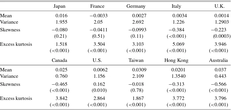
The full data period is divided into a learning sample: Janu-ary 1, 2001 to JanuJanu-ary 10, 2005; and a forecast sample: the 500 trading days from January 11, 2005 to early to mid-January, 2007. Small differences in end-dates across markets occurred due to different market-specific nontrading days. Table2shows summary statistics from the full sample of the percentage log returns of the market indices including sample mean, variance, skewness, and kurtosis. All 10 series display the standard prop-erties of daily asset returns: they are heavy tailed and mostly negatively skewed.
Parameter estimates from the T-CAViaR model are not shown to save space. However, for each dataset, the MCMC burn-in sample size is 15,000 iterations, followed by a sampling pe-riod of 25,000 iterations. To assess mixing and convergence, the MCMC method is run from five different, randomly gen-erated, starting positions, for each market, atα=0.01,0.05. The starting values of each of (β1, . . . , β6) were chosen to lie on either side of the estimated posterior mean. Convergence to the same posterior distribution is clear in all five runs for each parameter, in each case well before the end of the burn-in sam-ple, in each market. Gelman’s R statistics (see Gelman et al.
2005, p. 296) over these five runs, for the Australian market data, were between 1.002 and 1.040 over the six parameters: a typical result; all highlighting fast mixing and clear and effi-cient convergence for the proposed sampling scheme. Further, observed MH acceptance rates in these MCMC runs were be-tween 15% and 40%, which Gelman, Roberts, and Gilks (1996) note “yields at least 80% of the maximum efficiency obtain-able” for a Metropolis method. These figures are quite repre-sentative of the R values and observed MH acceptance rates during the sampling period across all markets.
Table 2. Summary statistics: percentage log returns on 10 market indices
Japan France Germany Italy U.K.
Mean 0.016 −0.0033 0.0027 0.0034 0.0014
Variance 1.955 2.05 2.692 1.226 1.2903
Skewness −0.080 −0.0411 −0.0993 −0.384 −0.223
(0.21) (0.51) (0.11) (<0.001) (0.0003)
Excess kurtosis 1.518 3.504 3.103 5.069 3.946
(<0.001) (<0.001) (<0.001) (<0.001) (<0.001)
Canada U.S. Taiwan Hong Kong Australia
Mean 0.025 0.0062 0.0309 0.0201 0.037
Variance 0.760 1.156 2.109 1.3540 0.443
Skewness −0.465 0.162 −0.018 −0.313 −0.566
(<0.001) (0.010) (0.78) (<0.001) (<0.001)
Excess kurtosis 3.842 2.864 1.867 3.772 3.796
(<0.001) (<0.001) (<0.001) (<0.001) (<0.001)
NOTE: Percentage log returns are analyzed.p-values based on asymptotic normality are listed, under a null hypothesis of 0 in each case.
7.1 Forecasting VaR Study
VaR is forecast one day ahead for each day in the forecast sample of 500 returns, using a range of competing models from all three quantile estimation classes: nonparametric, semipara-metric, and fully parametric. Many financial institutions use historical simulation to forecast VaR; we follow their approach and employ a short-term (ST, last 25 days) and a long-term (LT, last 100 days) percentile: these are nonparametric estimates. We compare two full T-CAViaR models: one with local return threshold (TCAV), the other with US market return threshold (TCAVx), with the two nested versions: AS and SAV, as well as a range of popular GARCH specifications, including
GARCH-n, GARCH-t; GJR-GARCH (GJR), and IGARCH. Except for the RiskMetrics (RMetrics) model, where the parameter is set to 0.94, all estimation uses MCMC methods. Details for the MCMC algorithms can be found in Chen, Gerlach, and So (2006). We also consider the MCMC method of Geweke and Keane (2007) (GK), that employs a smooth mixture of Gaussian regression models. This method requires a long presample pe-riod of returns: we use an extra 1000 daily returns, pre-2001, and the same settings as in Geweke and Keane (2007). For each dayyn+t in the forecast sample, parameters are estimated
for each semiparametric and parametric model, employing the entire previous data set (y1, . . . ,yn+t−1) as observations, then
forecasts are generated for the next day’sα-level quantile. Thus
25,000 (post burn-in) MCMC VaR forecasts are generated each day for each model. The posterior mean quantile forecast for each day is the average of these MCMC forecasts. Each MCMC run takes just under one minute on a standard modern desktop PC, so estimating two years of forecasts (500 days) takes ap-proximately 8 hours, for each model.
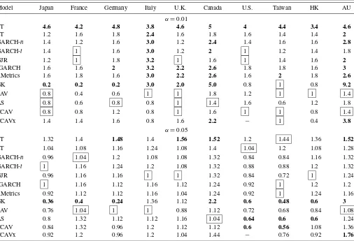
Table3 shows the ratios of the observed VRate to the true nominal level, forα=0.01,0.05, across all 12 models/methods and 10 markets. The best model’s ratio in each market is boxed, while bolding indicates the UC test rejects the model’s VRate, at the 5% level. The results are quite different fromα=0.01 to 0.05. First, atα=0.01, in all markets, except France, one of the CAViaR models ranks (at least equal) first, with VRate/α clos-est to 1. Further, the long and short-term HS methods, together with the full set of GARCH models, all have ratios mostly above 1 across the 10 markets. Thus, this group of models con-sistently under-estimates 1% risk levels in these markets. The GK method is highly variable in its VRate accuracy across the markets, at this level.
A different story applies atα=0.05. Here the models are much closer in performance, with first place rankings spread across models over the 10 markets, and ratios closer to 1 (in lo-cation and spread) across most models, compared toα=0.01. However, again both the GK method and the short-term per-centile method (ST) consistently under-estimate risk.
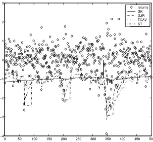
Figures 1 and2 illustrate some VaR forecasts for the Ital-ian MIBTel index returns at α=0.01,0.05, respectively. For
Table 3. Ratio of VRate/αatα=0.01,0.05 for each model across the 10 markets
Model Japan France Germany Italy U.K. Canada U.S. Taiwan HK AU
α=0.01
ST 4.6 4.2 4.8 3.8 4.6 5 4 4.4 3.4 4.6
LT 1.2 1.6 1.8 2.4 1.6 1.8 1.6 1.4 1.4 2
GARCH-n 1.4 1.2 1.6 3.0 1.2 2.4 1.4 1.6 1.6 2.8
GARCH-t 1.4 1 1.6 3.0 1.2 2 1 1.2 1.4 1.8
GJR 1.2 1 1.8 3.2 1 1.6 1 1.4 1.6 2
IGARCH 1.6 1.6 2 3.2 2.2 2.6 1.8 1.8 1.6 3
RMetrics 1.6 1.8 1.6 3.0 2.2 2.6 1.6 2 1.8 2.6
GK 0.2 0.2 0.2 3.0 2.0 5.0 0.8 1 0.8 9.2
SAV 0.8 0.4 0.6 1 1 1.8 1.2 1 1 1.4
AS 0.8 0.6 0.8 0.8 1 1.4 1.6 0.6 1.2 1.8
TCAV 0.8 0.8 1.2 0.8 1 1.6 1 1 0.8 1.4
TCAVx 1.4 1.4 1.6 0.8 1.6 2.2 − 1 0.4 3.8
α=0.05
ST 1.32 1.4 1.48 1.4 1.56 1.52 1.2 1.44 1.36 1.52
LT 1.04 1.08 1.16 1.24 1.08 1.4 1.04 1.2 1.08 1.28
GARCH-n 0.96 1.04 1.2 1.08 1.08 1.32 0.84 0.84 1.16 1.32
GARCH-t 1 1.16 1.24 1.2 1.08 1.32 0.88 0.88 1.2 1.32
GJR 0.96 1.16 1.16 1 1 1.32 0.84 0.72 1 1.24
IGARCH 1 1.16 1.12 1.16 1.12 1.24 0.92 1 1.2 1.2
RMetrics 0.92 1.12 1.12 1.16 1.04 1.24 0.92 1 1.24 1.16
GK 0.36 0.4 0.24 1.36 1.12 2.2 0.6 0.48 0.6 3
SAV 0.76 1.04 1 1 0.88 1.12 0.72 0.68 0.84 1.08
AS 0.8 1.32 1.12 1.12 1.16 1.04 0.64 0.6 0.6 1.24
TCAV 0.84 1.32 0.96 1.2 1.12 1.12 0.6 0.56 1.08 1.36
TCAVx 0.92 1.2 0.96 1.2 1.04 1.44 − 0.76 0.92 1.76
NOTE: Boxes indicate closest to 1 in that market, bold indicates the model is rejected by the unconditional coverage test (at a 5% level), for each market. AU: Australia.
Figure 1. Italian MIBTel index returns January 2005 to January 2007 (circles), together with four sets of forecasted VaR series atα=0.01. Series are GK, GJR, TCAV, and ST.
Figure 2. Italian MIBTel index returns January 2005 to January 2007 (circles), together with four sets of forecasted VaR series atα=0.05. Series are GK, GJR, TCAV, and ST.
Italy, atα=0.01 the four CAViaR models ranked first-fourth in VRate/0.01 with 1 (SAV) and 0.8 (AS, TCAV, TCAVx), fol-lowed by the GARCH and GK models with ratios, all signifi-cantly different to 1, of 3 (GJR and GK) or 3.2; while the ST method had a ratio of 3.8. Figure1highlights that the T-CAViaR model was clearly more extreme (and accurate) in its quantile forecasts in this market. The GARCH models’ VaR forecasts, similar to the GJR shown, are consistently not large enough in magnitude for a 1% quantile level, compared to the actual returns being forecast. The GK method, while demonstrating that it can capture heteroscedasticity, seemed too smooth in its dynamic quantiles for this market, and did not produce VaR forecasts that reacted to high volatility periods as much as the other models/methods did, its quantile forecasts being less ex-treme than all other methods in highly volatile return periods and being generally much smoother. The ST method is clearly not optimal for this market either, partly since 25 days is not sufficient to estimate a 1% sample quantile. ST’s forecasts are far less smooth than all other models in this case.
Figure 2 shows the VaR forecasts for α=0.05, again for Italy, and for the same four methods. Now we see that the ST method, at least in low-medium volatility periods, is approx-imating the GARCH (all similar to the GJR shown) models’ forecasts, which are all quite similar to the T-CAViaR model. However, the ST method “recovers” slowest after extreme re-turns or high volatility periods, since any extreme return will af-fect the sample percentile for exactly 25 days. The GK method’s VaR forecasts again seem quite different to the other methods: it is smoother and less reactive to extreme returns. Though it can clearly capture some types of heteroscedasticity, it struggled to accurately capture the specific dynamic volatility process in this data set, at bothα=0.05,0.01.
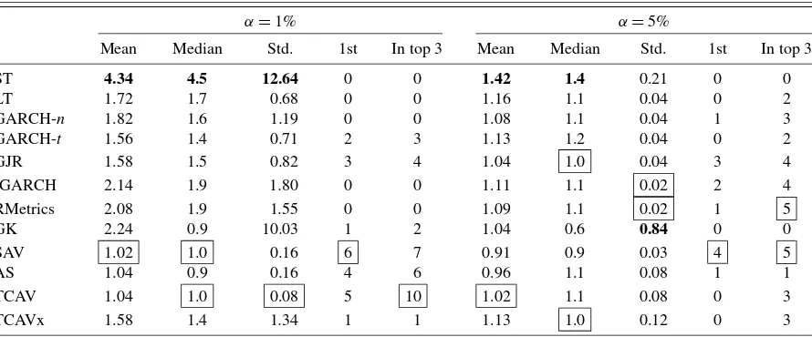
Table4displays summary statistics for the observed VRate/α ratios for each model across the 10 markets, using the numbers in Table3. The ‘Std.’ labeled column shows the standard devi-ation from the expected ratio of 1 (not the sample mean), while ‘1st’ counts the markets where that model had VRate ratio clos-est to 1 and ‘In top 3’ counts the markets where the model
ranked in the top 3 models by VRate ratio. The results confirm and add to the conclusions above. At α=0.01 the SAV, AS and TCAV (self-exciting) models are most favored across all criteria. In particular, their ratios VRate/αare very close to 1, both in location and spread, and they mostly rank in the top three models for each market. The GARCH models considered all under-estimate risk, with ratios above 1 in most markets, as also do the GK and HS methods. The TCAV model has the low-est deviation in ratios away from 1, average ratio second closlow-est to 1, and is ranked in the top 3 models for all 10 markets. The SAV ranks first in six markets, has average ratio closest to 1, had second lowest deviation in ratios and finished in the top 3 models in seven markets.
Table4shows that all the models atα=0.05 have ratios that average close to 1 across markets, except the short-term 25 day percentile (ST), with small deviations away from 1 (except the GK method). The GARCH and CAViaR models are quite com-parable at this risk level, and are hard to distinguish between: the TCAV model has average ratio closest to 1, followed by the AS and GJR models. However, again the SAV has the most firs rankings, with four markets, and, together with RMetrics, the most top three rankings, with five markets. The fully threshold CAViaR models both have larger deviations in ratios than the RMetrics, IGARCH, GARCH, ST, LT, AS, and SAV models. The RMetrics and IGARCH models have the lowest deviation in ratios from 1, closely followed by the SAV model. If a con-servative risk model is preferred, the SAV is the best candidate, with mean and median ratios at 0.9 and third lowest deviation in ratio from 1.
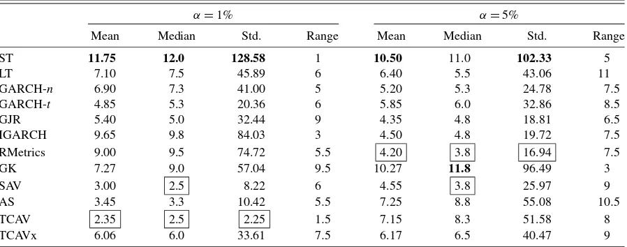
To help distinguish between the better models at each quan-tile level, Table 5 shows summary statistics for each model’s rank in terms of how close its VRate/α ratio is to 1, across the markets. For ratios that are equidistant from 1, conserva-tive ratios (less than 1) are preferred. Table5displays the aver-age, median, standard deviation (from 1) and range of the fore-cast ranks for each model over the ten markets. At α=1%, the self-exciting T-CAViaR model has by far the lowest mean rank, equal lowest median rank, and by far the smallest de-viation in ranks, away from 1, across the models. In fact, the
Table 4. Summary statistics for VRate/αatα=0.01,0.05 for each model across the 10 markets
α=1% α=5%
Mean Median Std. 1st In top 3 Mean Median Std. 1st In top 3
ST 4.34 4.5 12.64 0 0 1.42 1.4 0.21 0 0
NOTE: Boxes indicate the favored model, bold indicates the least favoured model, in each column; ‘Std.’ is the standard deviation in ratios from an expected value of 1; ‘1st’ indicates the number of markets where that model’s VRate ratio ranked closest to 1; ‘In top 3’ counts the number of markets where the model’s VRate ratio ranked in the top 3 models.
Table 5. Summary statistics for model ranks, in terms of VRate/α, atα=0.01,0.05 across the 10 markets
α=1% α=5%
Mean Median Std. Range Mean Median Std. Range
ST 11.75 12.0 128.58 1 10.50 11.0 102.33 5
LT 7.10 7.5 45.89 6 6.40 5.5 43.06 11
GARCH-n 6.90 7.3 41.00 5 5.20 5.3 24.78 7.5
GARCH-t 4.85 5.3 20.36 6 5.85 6.0 32.86 8.5
GJR 5.40 5.0 32.44 9 4.35 4.8 18.81 6.5
IGARCH 9.65 9.8 84.03 3 4.50 4.8 19.72 7.5
RMetrics 9.00 9.5 74.72 5.5 4.20 3.8 16.94 7.5
GK 7.27 9.0 57.04 9.5 10.27 11.8 96.49 3
SAV 3.00 2.5 8.22 6 4.55 3.8 25.97 9
AS 3.45 3.3 10.42 5.5 7.25 8.8 55.08 10.5
TCAV 2.35 2.5 2.25 1.5 7.15 8.3 51.58 8
TCAVx 6.06 6.0 33.61 7.5 6.17 6.5 40.47 9
NOTE: Boxes indicate the favored model, bold indicates the least favored model, in each column; ‘Std.’ is the standard deviation in ranks from the value of 1.
TCAV model ranks in the top 3 in every market, and thus has the smallest range in ranks (except for ST which only ranked 11th or 12th). The SAV and then AS CAViaR models are next best, with SAV having the equal best median rank and 2nd best mean rank and 2nd lowest deviation in ranks, and the AS model finishing 3rd on mean, median, and deviation in rank mea-sures. The GARCH-n, GARCH-t, GJR-GARCH, and TCAVx models typically ranked just behind the TCAV, SAV, and AS CAViaR models in 4th–7th placing in each market, followed by the long-term percentile (LT) and GK methods; while RMet-rics, IGARCH and short-term (ST) percentile methods typically ranked in the last three places in each market. Clearly the TCAV model has forecast dynamic quantiles accurately and compar-atively the best over the twelve models and 10 markets con-sidered, atα=0.01. Further, three of the CAViaR models do best as a group, followed by the stationary GARCH specifica-tions, the GARCH-t’s fat-tails outperforming the GARCH-n as expected, then the TCAVx, GK and remaining methods. Risk-Metrics and IGARCH do not forecast VaR well at this quantile level at all, nor did the HS methods.
Forα=0.05, the RiskMetrics method now has the lowest average and equal lowest median rank across markets, closely followed by the GJR-GARCH, IGARCH, and SAV models in mean rank. The RMetrics method also has the lowest deviation in ranks away from 1. Clearly, no model dominated in rank, and thus risk ratio accuracy, at this risk level, since the summary rank measures are above 4 in average and have much larger deviation, compared to those for α=0.01. The SAV model finished with the equal best median rank and 4th best in both mean and standard deviation in ranks across markets. These four models are hard to separate at this quantile level, but the RiskMetrics method is marginally favored considering both Ta-bles4and5. The AS and T-CAViaR models now typically rank in the middle (i.e., 6th to 9th) of the 12 models.
To summarize, the fully nonlinear self-exciting T-CAViaR model is favored for accurate dynamic quantile forecasting whenα=0.01, ranking first in all summary rank measures and first in median and deviation in VRate ratios from 1; followed by the SAV and AS CAViaR models. Further, atα=0.05, four models: RMetrics, GJR, IGARCH, and SAV, are hard to sep-arate, though RMetrics could be favoured since it ranked first
in all summary rank measures and had equal lowest deviation in VRate ratios. We now formally test these models, as a final point of comparison.
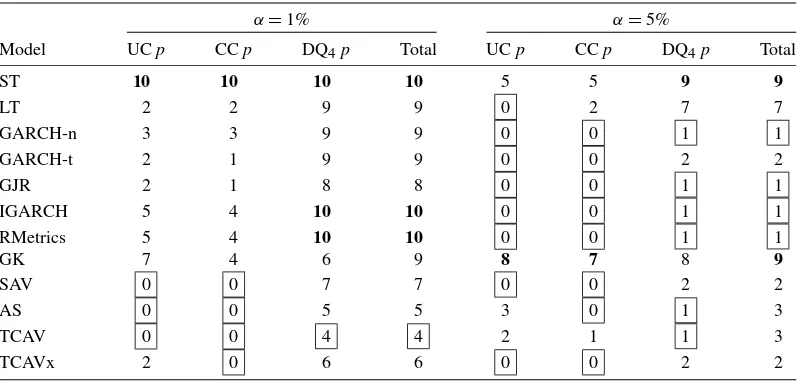
Table6counts the number of rejections for each model, over the 10 markets, at the 5% significance level, for each of the three tests considered: UC, CC, and the DQ tests. Four lags were used, as in Engle and Manganelli (2004). Atα=0.01 most of the models are rejected in most of the markets, mainly by the DQ test. The CAViaR models fare best as a group, with the self-exciting T-CAViaR model rejected in the least number of markets for all three tests, and for all tests combined (four re-jections across 10 markets), followed by AS with five, TCAVx with six, and SAV with seven rejections. The GK method is only rejected in six markets by DQ, but in nine markets overall, while all the GARCH models are rejected in at least eight mar-kets; ST, RMetrics, and IGARCH are rejected in all 10 markets. Atα=0.05 the HS (ST, LT) and GK methods are rejected in seven or nine markets, while the CAViaR models are rejected in two or three markets each; the GARCH and RMetrics models fare best with only 1 or 2 rejections across markets.
In summary, the CAViaR family of models are highly com-petitive at worst, and far more accurate at best, at dynamic quan-tile VaR forecasting, compared to a range of popular and well-known VaR methods. At α=0.05 most of the models fore-casted similarly with no clear standout, though RiskMetrics and the CAViaR SAV model finished best in mean and median rank-ing, respectively, in terms of violation rates, across markets; and the RiskMetrics, GJR and GARCH-nmodels are rejected the least across all VaR forecast methods. The full T-CAViaR model, though still performing well in overall violation rate across markets, is perhaps an unnecessarily complex model at quantile level 0.05, the simpler symmetric models fared better at this level. However, the self-exciting T-CAViaR model per-formed in a comparably superior fashion to the other models, followed by the remaining CAViaR specifications, forα=0.01. Its VaR forecasts display violation rates that are consistently closest to nominal and the model is rejected the least number of times across the 10 markets. The RiskMetrics, IGARCH, sta-tionary GARCH, GK, and HS methods are simply not com-petitive with the CAViaR models at forecasting risk levels or
Table 6. Counts of model rejections for three standard quantile coverage tests, across the 10 markets
NOTE: Boxes indicate the favored model, bold indicates the least favored model, in each column.
dynamics, at this more extreme quantile: all over-estimated the risk levels and/or do not effectively capture the dynamics of risk and are subsequently rejected by the formal tests, especially the DQ test, in most markets atα=0.01.
8. CONCLUSION
This article proposes a new fully nonlinear CAViaR model for dynamic quantile estimation. Bayesian MCMC methods are adapted to this family, employing the well-known link between the quantile estimation criterion function and the Skewed-Laplace density. MCMC estimation proves favourably precise and efficient, in simulations from a GARCH model, compared to the classical numerically optimized quantile criterion func-tion, at the quantile levels 0.05 and 0.01. A VaR forecasting study reveals that the fully nonlinear self-exciting T-CAViaR model compares most favorably in terms of violation rates and independence of violations, to more parsimonious CAViaR models at level 0.01, while the simplest CAViaR SAV model fares better than the nonlinear CAViaR models at level 0.05. A range of well-known GARCH models, including RiskMet-rics, historical simulation and a semiparametric smoothly mix-ing regression approach are not competitive at the quantile level 0.01, across the 10 markets. However, at level 0.05, most mod-els forecast reasonably similarly, with results marginally favor-ing simpler specifications such as RiskMetrics, GJR-GARCH, and the CAViaR SAV specification.
ACKNOWLEDGMENTS
We thank an AE and an anonymous referee for their insight-ful and helpinsight-ful comments and suggestions which improved the article. Cathy Chen is supported by the grant 96-2118-M-002-MY3 from the National Science Council (NSC) of Taiwan. The revision of this article was conducted while Richard Gerlach was a Visiting Scholar at Feng Chia University supported by the Mathematics Research Promotion Center, NSC, Taiwan.
[Received July 2008. Revised January 2010.]
REFERENCES
Berkowitz, J., Christoffersen, P., and Pelletier, D. (2010), “Evaluating Value-at-Risk Models With Desk-Level Data,”Management Science, to appear. [486]
Black, F. (1976), “Studies in Stock Price Volatility Changes,” inProceedings of the Business and Economic Statistics Section, Alexandria, VA: American Statistical Association, pp. 177–181. [481,483]
Bollerslev, T. (1986), “Generalized Autoregressive Conditional Heteroskedas-ticity,”Journal of Econometrics, 31, 307–327. [481]
Brooks, C. (2001), “A Double-Threshold GARCH Model for the French Franc/Deutschmark Exchange Rate,”Journal of Forecasting, 20, 135–143. [481,483]
Chen, C. W. S., and So, M. K. P. (2006), “On a Threshold Heteroscedastic Model,”International Journal of Forecasting, 22, 73–89. [481,484] Chen, C. W. S., Gerlach, R., and So, M. K. P. (2006), “Comparison of
Non-Nested Asymmetric Heteroskedastic Models,”Computational Statistics and Data Analysis, 51 (4), 2164–2178. [487]
Christoffersen, P. (1998), “Evaluating Interval Forecasts,”International Eco-nomic Review, 39, 841–862. [486]
Engle, R. F. (1982), “Autoregressive Conditional Heteroskedasticity With Es-timates of the Variance of United Kingdom Inflations,”Econometrica, 50, 987–1007. [481]
Engle, R. F., and Manganelli, S. (2004), “CAViaR: Conditional Autoregressive Value at Risk by Regression Quantiles,”Journal of Business & Economic Statistics, 22, 367–381. [481,483,486,490]
Gelman, A., Carlin, J. B., Stern, H. S., and Rubin, D. B. (2005),Bayesian Data Analysis(2nd ed.), Boca Raton, FL: Chapman & Hall. [484,486] Gelman, A., Roberts, G. O., and Gilks, W. R. (1996), “Efficient Metropolis
Jumping Rules,” inBayesian Statistics 5, Oxford: Clarendon, pp. 599–608. [484,486]
Geraci, M., and Bottai, M. (2007), “Quantile Regression for Longitudinal Data Using the Asymmetric Laplace Distribution,” Biostatistics, 8, 140–154. [481]
Geweke, J., and Keane, M. (2007), “Smoothly Mixing Regressions,”Journal of Econometrics, 138, 252–290. [481,487]
Giacomini, R., and Komunjer, I. (2005), “Evaluation and Combination of Con-ditional Quantile Forecasts,”Journal of Business & Economic Statistics, 23, 416–431. [481]
Glosten, L. R., Jagannathan, R., and Runkle, D. E. (1993), “On the Relation Be-tween the Expected Value and the Volatility of the Nominal Excess Return on Stock,”Journal of Finance, 48, 1779–1801. [483]
Hastings, W. K. (1970), “Monte-Carlo Sampling Methods Using Markov Chains and Their Applications,”Biometrika, 57, 97–109. [484]
Jorion, P. (1996), “Risk: Measuring the Risk in Value at Risk,”Financial Analy-sis Journal, 52, 47–56. [481,482]
Koenker, R., and Bassett, G. (1978), “Regression Quantiles,”Econometrica, 46, 33–50. [481]
Kuester, K., Mittnik, S., and Paolella, M. S. (2006), “Value-at-Risk Prediction: A Comparison of Alternative Strategies,”Journal of Financial Economet-rics, 4, 53–89. [481]
Kupiec, P. H. (1995), “Techniques for Verifying the Accuracy of Risk Measure-ment Models,”Journal of Derivatives, 3, 73–84. [486]
Li, C. W., and Li, W. K. (1996), “On a Double-Threshold Autoregressive Het-eroscedastic Time Series Model,”Journal of Applied Econometrics, 11, 253–274. [483]
Manganelli, S., and Engle, R. F. (2004), “A Comparison of Value-at-Risk Mod-els in Finance,” inRisk Measures for the 21st Century, ed. G. Szegö, Chich-ester: Wiley. [481,482]
Metropolis, N., Rosenbluth, A. W., Rosenbluth, M. N., Teller, A. H., and Teller, E. (1953), “Equation of State Calculations by Fast Computing Machines,”
Journal of Chemical Physics, 21, 1087–1092. [484]
Morgan, J. P. (1996),RiskMetrics—Technical Document(4th ed.), New York: Morgan Guaranty Trust Company. [482]
Nelson, D. B. (1991), “Conditional Heteroskedasticity in Asset Returns: A New Approach Econometrica,”Econometrica, 59, 347–370. [483]
Tong, H. (1978), “On a Threshold Model” inPattern Recognition and Signal Processing, ed. C. H. Chen, Amsterdam: Sijhoff & Noordhoff. [483]
(1983),Threshold Models in Non-Linear Time Series Analysis. Lecture Notes in Statistics, Vol. 21, New York: Springer-Verlag. [483]
Tsay, R. S. (2005),Analysis of Financial Time Series(2nd ed.), Hoboken: Wi-ley. [482]
Tsionas, E. G. (2003), “Bayesian Quantile Inference,”Journal of Statistical Computation and Simulation, 9, 659–674. [481,482]
Wong, C. M., and So, K. P. (2003), “On Conditional Moments of GARCH Models, With Applications to Multiple Period Value at Risk Estimation,”
Statistica Sinica, 13, 1015–1044. [486]
Yu, K., and Moyeed, R. A. (2001), “Bayesian Quantile Regression,”Statistics and Probability Letters, 54, 437–447. [481-483]
Yu, P. L. H., Li, W. K., and Jin, S. (2010), “On Some Models for Value-at-Risk,”
Econometric Reviews, to appear. [483]
Zakoian, J. (1994), “Threshold Heteroskedastic Model,”Journal of Economic Dynamics and Control, 18, 931–955. [481,483]