Chapter 1
Introduction to Graph Theory
D r . Al i Ma h m u d i ( Ju r u sa n Pen d i d i k a n M a t em a t i k a FM I PA U NY)
To those who ask what the infinitely small quantity in mathematics is, we answer that it is actually zero. Hence there are not so many mysteries hidden in this concept as they are usually believed to be.
(Leonhard Euler (1707-1783)
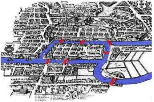
A. The Konigsberg Problem
Konigsberg is a city which was the capital of East Prussia but now is known as Kaliningrad in Russia. The city is built around the River Pregel where
it joins another river. An island named Kniephof is in the middle of where the
two rivers join. There are seven bridges that join the different parts of the city on
both sides of the rivers and the island as shown in the Figure 1.1.
(Sumber: http://math.youngzones.org/Konigsberg.html)
People tried to find a way to walk all seven
bridges without crossing a bridge twice. This
problem was called Konigsberg bridge problem: is
there a walking route that crosses each of the
seven bridges of Konigsberg exactly once? The
problem came to the attention of a Swiss
mathematician named Leonhard Euler
(pronounced "oiler").
In 1735, Euler presented the solution to the problem. He explained why
crossing all seven bridges without crossing a bridge twice was impossible. While
solving this problem, he developed a new mathematics field called graph theory,
which later served as the basis for another mathematical field called topology.
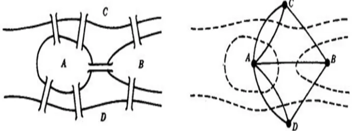
The key to Euler’s solution was very simple abstraction of the problem. Euler
redraw the diagram of the city of Konigsberg by representing each of the land
masses as a vertex and representing each bridge as an edge connecting the vertices
corresponding to the land masses as shown in the Figure 1.2. By this method we
have a graph that encodes the necessary information. The problem reduces to
finding a “closed walk” in the graph which traverses each edge exactly once. This
is called an Eulerian circuit.
Figure 1.2. Graph as a Model of Konigsberg Problem Leonhard Euler (1707-1783)
The field of graph theory began to blossom in the twentieth century as more
and more modeling possibilities we recognized – and growth continues. In the
mid 1800s, people began to realize that graphs could be used to model many
things that were of interest in society. For example, the “Four Color Maps
Conjecture”, introduced by DeMorgan in 1852, was a famous problem that was seemingly unrelated to graph theory. The conjecture stated that four is the
maximum number of colors required to color any map where bordering regions
are colored differently. This conjecture can easily be phrased in terms of graph
theory, and many researchers used this approach during the dozen decades that the
problem remained unsolved.
B. The Definition of Graph
In a football league there are eight teams, which we denote by A, B, C, D, E,
F, G, and H. After a few weeks of the season the following games have been
played.
A has played F and H
B has played E, F, and H C has played G and H
D has played E and G
E has played B, D, and G
F has played A and B G has played C and E
H has played A, B, and C
We may illustrate this situation by either of the two diagram of Figure 1.3,
where the teams are represented by dots and two such dots are joined by a line
whenever the corresponding teams have played each other.
Figure 1.3. Games in the Football League
A B
C
D
E F
G H
A B
C
D
E F
In the diagram on the left, the dots have been joined using straight lines,
while in the other diagram three of lines used are not straight. But since we are
only interested in which games have been played, it does not matter whether the
lines are straight or not.
The diagrams may be used to describe other situation. For example, the
eight dots represent eight people, with le line joining a pair of dots if the two
people know each other. Or, the dots could be communication centre with the
lines denoting communication links. Indeed, as we will see later, many real-world
situations can conveniently be described by means of such drawing, which we call
graphs. A graph can be thought of as a drawing or diagram consisting of
collection of vertices (dots or points) together with edges (lines) joining certain
pairs of these vertices, as in the diagrams of Figure 1.2. Here is formal definition
of graph.
If u and v are two vertices in G and e = (u,v) is edge in G, then
(i) vertex u and v are endpoints of edge e
(ii) vertex u and v are adjacent
(iii) vertex u and v incident to e or e incident to vertex u and v
Consider that both graph of Figure 1.3 represent an equal graph. The vertex
set of the graph is V = {A, B, C, D, E, F, G, H} and the edge set is E = {(A,F),
(A,H), (B,E), (B,F), (B,H), (C,G), (C,H), (D,E), (D,G), (E,G)}. We can also notate
the edge set as E = {AF, AH, BE, BF, BH, CG, CH, DE, DG, EG}. Definition 1.1
A graph G = ((V(G), E(G)) consist two sets, V(G) and V(G). V(G) is the vertex
set of the graph, often denoted by just V, which is a nonempty set of elements
called vertices. E(G) is the edge set of the graph, often denoted by just E, which
is a possibly empty set of elements called edges, such that each edge e in E is
Example 1.1
Let G = (V(G), E(G)) is a graph, where V(G) = {1, 2, 3, 4} and E(G) = {(1,2),
(1,3), (1,4), (2,4)}. We can represent the graph as follow.
Figure 1.4. A Graph with Four Vertices and Five Edges
C. Graph as a Model
Graph theory provides a natural mathematical model for some problems. At
this chapter we only describe the problem and delay detailed discussion of their
solution to later chapters.
Problem 1
Suppose that the graph of Figure 1.5 represents a network of telephone lines and
poles. We are interested in the networks vulnerability to accidental disruption. We
want to identify those lines and poles that must stay in service to avoid
disconnecting the network.
Figure 1.5. Network of Telephone Line 2 1
4 3
D A
B
C
E
F e1
e2
e3 e4
e5
e6
There is no single line whose disruption (removal) will disconnect the graph
(network), but the graph will become disconnected if we remove the two lines
represented by edges e4 and e5, for example. When it comes to poles, the network is more vulnerable since there is a single vertex, vertex d, whose removal
disconnects the graph. This illustrates the notions of edge connectivity and vertex
connectivity of a graph.We may also want to find a smallest possible set of edges
needed to connect the six vertices. There are several examples of such minimal
sets. One is {e1, e3, e5, e6, e7}
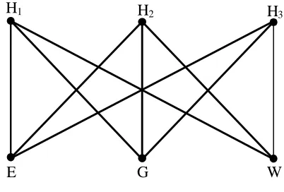
Problem 2
Suppose we have three houses each of which have to be supplied with electricity,
gas and water. Is it possible to connect each utility with each of the three houses
without the lines or mains crossing?
We can represent the connection of the three houses to the three utilities by
the graph of Figure 1.6. Here we have a graph with six vertices, three of which
represent the houses (denoted by H1, H2, H3), the other three represent the utilities (denoted by E, G, W), and an edge joins two vertices if and only if one vertex
denotes a house and the other vertex a utility.
Figure 1.6 The Three Utilities Graph
The problem then is as the whether or not we can draw this graph in such a
way that no two edges intersect. The answer is no – we will see why when we
look at planar graphs in Chapter 4. E
H1 H2 H3
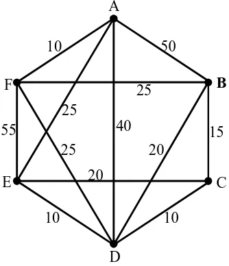
Problem 3
A company has branches in each of six cities C1, C2, C3, …, C6. The airfare for a
direct flight from Ci to Cj is given by the (i, j)th entry of the following matrix (where indicates that there is no direct flight). For example the fare from C1 to
C4 is IDR 400.000,00 from C2 to C3 is IDR 1.500.000,00.
pairs of cities. (Even if there is a direct flight between two cities this may not be
the cheapest route). We can first represent the situation by a weighted graph, i.e., a
graph with “weights” attached to edges according to the airfares, as in Figure 1.7.
Figure 1.7 The Weighted Graph of Airfare for Direct Flights Between Six Cities
The problem can then be solved using Dijkstra’s algorithm. This type of
D. Some Type of Graphs
Note that in the definition of graph, we do not exclude the possibility that
the two endpoints of an edge are the same vertex. This called loop, for obvious
reasons. Also, we may have multiple edges, which is when more than one edge
shares the same set of endpoints, i.e, the edges of the graph are not uniquely
determined by their endpoints. In another word, two (more) edges that have end
vertices are called multiple edges or parallel edges.
A vertex of a graph which is not the end of any edge is called isolated. Two
vertices which are joined by an edge are said to be adjacent or neighbors. The set
of all neighbors of a fixed vertex v of G is called the neighborhood set of v and is
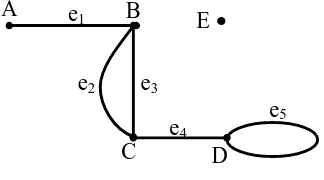
denoted by N(v). Given graphs G= (V(G), E(G)), where V(G) = {v1, v2, v3, v4} and E(G1) = {v1v2, v1v3, v3v4}. We can graphically represent this graph in Figure 1.8 below.
Figure 1.8. Graph with multi edges, loop, and isolated vertex
In the graph in Figure 1.8, e2 and e3 are multiple-edges, edge e5 is loop, and E is an isolated vertex. The neighborhood of vertex B, D, and E, are N(B) = {A,
C}, N(D) = {C}, and N(E) = { } respectively.
1. Simple Graph and Multi-Graph E
D C
B A
e2 e3 e1
e5 e4
Definition 1.2
A graph is called simple if it has no loops and no multi-edges. In a simple graph, we often identify an edge using its endpoints, e.g, edge (u, v).
2. Complete Graph
If the complete graph has vertices v1, v2, …, vn then the edge set can be given by
E = {(vi, vj); vi vj; i,j = 1, 2, …, n}
Note that the grah has n
n 1 21
edges, since there are n – 1 edges incident
with each of the n vertices vi, so a total of n(n – 1), but divide by 2, since (vi, vj) = (vj, vi). A complete graph with n vertices is denoted by Kn. Figure 1.9 shows K1,
K2, …, K5.
Figure 1.9 The Complete Graphs on at most five vertices
3. Empty Graph
K1 K2
K4 K
5
K3 Definition 1.3
A complete graph is a simple graph in which each pair of distinct vertices
is joined by an edge.
Definition 1.4
An empty graph with n vertices is denoted by Nn. Figure 1.10 shows N1, N2,
…, N5.
Figure 1.10 The Null Graphs on at most five vertices
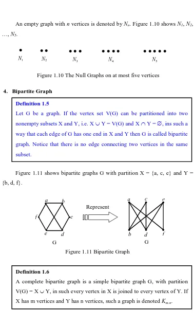
4. Bipartite Graph
Figure 1.11 shows bipartite graphs G with partition X = {a, c, e} and Y =
{b, d, f}.
Figure 1.11 Bipartite Graph
G
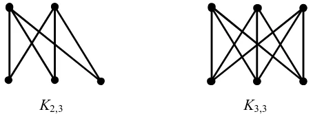
Consider that since each of the m vertices in the partition set X of Km,n is
adjacent to each of the n vertices in the partition set Y, Km,n has m x n edges.
Figure 1.12 shows complete bipartite graphs K2,3 and K3,3.
Figure 1.12 Complete Bipartite Graph
Proof
Suppose a graph contains a triangle {u, v, s}. By definition, we have edges uv, vs,
and su.
We prove the graph is not bipartite by contradiction.
Assume that it is bipartite. Then we can have a partition {U, V} of vertex set.
Consider which of the two subsets U, V each of the three vertices u, v, s belongs.
Clearly, there must be at least two vertices among u, v, s belonging to the same
subset, which means there is no edge connecting them.
Contradiction.
E.Vertex Degrees
K2,3 K3,3
Theorem 1.1
A graph is not bipartite if it contains a triangle. (A triangle in a graph is three
vertices such that any two of them are neighbors.
Denition 1.5
Let v be a vertex of the graph G. The degree of v, denoted by d(v) or dG(v), is the number of edges of G incident with v, counting each loop twice, i.e, it is
Minimum and maximum degree of G, denoted (G) dan (G) respectively,
are defined below.
(G) = minimum {d(v) | v V(G)}
(G) = maxsimum {d(v) | v V(G)}
Consider Figure 1.13 below.
Figure 1.13
twice. (Note that even a loop contributes 2 although the 2 ends are identical).
Notice that in the Figure 1.13 there is an even number of odd vertices. A
vertex of a graph is called odd or even depending on whether its degree is odd or
even.
Theorem 1.2 Handshaking Theorem
For any graph G
Proof
d is even (being the difference of two even numbers).
As all the terms in
number of them (because the sum of an odd number of odd number is odd.
Corollary 1.3
In any graph G there is an even number of odd vertices
A complete graph is one that is k-regular for some k. The graph drawn
below graph G is a 2-regular and graph K4 is a 3-regular.
Figure 1.14 Regular.Graph
Notice that the complete graph Kn is (n-1)-regular. The complete bipartite
graph Kn,n is n-regular.
F. Isomorphic Graphs
It is often the case that two graphs have the same structure, differing only in
the way their vertices and edges are labeled or only in the way they are
represented geometrically. For many purposes, we can regard the two graphs as
essentially the same. This essential likeness has a special name and we now define
this formally.
In other word, the graphs G1 and G2 are isomorphic if the vertices of G1 can be paired off with the vertices of G2 and the edges of G1 can be paired off with the edges of G2 in such way that the ends paired off edges are paired off. Thus G1 is really just the same graph as G2, apart from a possible change in how the vertices
2-regular 3-regular
Definition 1.6
and edges are named (or a possible redrawing of the graphs). Figure 1.8 shows
five fairly obvious pairs of isomorphic graphs.
(a)
(b)
Figure 1.15 Isomorphic Graphs
Figure 1.15 gives some examples to illustrate that often it can be quite
difficult to determine if two graphs are isomorphic. In the Figure 1.15 (a) an
isomorphism is given by the following one-to-one correspondence of vertices:
A P, B Q, C R, D S
Note how A is joined with B and C, but not to D and similarly P is joined to
Q and R, but not to S.
The problem of determining when two graphs are isomorphic gets harder as
the number of vertices and edges of the graphs get larger. Clearly, if two graphs
G1 and G2 are isomorphic then they must have (i) The same number of vertices
(ii)The same number of edges A
B C
D
P
Q R
However, as we will now see, both conditions are not sufficient. The graph
G of Figure 1.16 has the same number of vertices and edges as the graph in Figure
1.15 (a), but G is not isomorphic to these graphs.
Figure 1.16
G. SubGraphs
Fo example, in Figure 1.17 H1 is subgraph of H and H2 is spanning subgraph of G.
Figure 1.17 Graph and Subgraph 1
H H2
K
L N
M
Definition 1.7
Let H be a graph with vertex set V(H) and an edge set E(H). Similarly let G be
a graph with vertex set V(G) and edge set E(G). H is called subgraph of G if
V(H) V(G)and E(H)E(G).
If V(H) = V(G) then H is spanning subgraph of G.
We also say that G is a supergraph of H.
G
Z X
V W V W
Z X
Y
Z
X
W V
Y
From the definition we can conclude that any simple graph on n vertices is
subgraph of the complete graph Kn. Notice that we can get a subgraph of any graph by deleting of a vertex or an edge the graph.
H. Complement of Graph
In the Figure below, Gc is complement of G.
Figure 1.18 Graph and Complement
Consequently If G is a complete graph, then Gc is a empty or null graph and for any graph, G Gc is a complete graph.
I. Representation of Graph
We can represent a simple graph G = (V(G),E(G)) in many different ways.
We have seen that we can represent it by describing V and E, or by drawing the
graph. Another possible representation is an adjacency matrix. Definition 1.8
Let G a simple graph. Complement of G, denoted Gc, is a simple graph in such that (V(G) = V(Gc)) and two vertices u is adjacent to v in Gc if and only if u is not adjacent to v in G
A
E B
D C
A
B
C D
E
1. Adjacency Matrix
Let G a graph with V(G) =
v1,v2,v3,...vn
. Adjacency matrix of G is a(symmetric) matrix A(G) =
aij , where a state the number of edges adjacent to ijvertices viand v . j
2. Incidency Matrix
Let G a graph with n vertices v1, v2, …, vn and k edges. Incidency matrix of G is a matrix I(G) =
mij that has ordo n x k, where:0, if edge ej is not incident to vertex vi
mij = 1, if edge ej incident to vertex vj and ej is not loop 2, if edge ej incident to vertex vi and ej is loop
Let G a graph represented by diagram below.
Figure 1.19
Adjacency matrix and incidency of graph G above are as follows
v1 v2 v3 v4 v1 1 1 2 0 A(G) = v2 1 1 1 1
v3 2 1 0 0 v4 0 1 0 0
e1 e2 e3 e4 e5 e6 e7 v1 2 1 1 1 0 0 0 v2 0 1 0 0 1 2 1 M(G) = v3 0 0 1 1 1 0 0 v 0 0 0 0 0 0 1
G
e1 v1
e4 e2 e3
e7 e5
e6
v3 v2
Based on the examples above we can notice the following characteristic.
1. Adjacency matrix is symmetric to main diagonal
2. If a graph has no loop, then each element of diagonal of adjacency matrix is
zero.
3. Element of matrix of simple graph is 0 or 1
4. Degree of vertex vi in G correspond to sum of all element of row (column) i of adjacency matrix if element of main diagonal i is multiplied by 2.
5. Degree of vertex vi in G correspond to sum all element of row i of incidency matirx
6. Sum all element of every column of incidency matrix is 2.
Exercise
1. Given graph G below.
a. Give a label to vertices of the graph
b. Determine a vertex and a edge set of the graph
c. Is this a simple graph?
2. Give an example of graph with 5 vertices, 5 edges, and 1 isolated vertex. Is
this a simple graph?
3. Give an example of graph with 4 vertices, 6 edges, and 1 isolated vertex. Is
this a simple graph?
4. A graph G has 17 vertices and.maximum vertex degree of G is 3. Determine
the maximum number of edges of G.
5. A graph G has 23 edges and minimum vertex degree of G is 5. Determine
minimum the number of vertices of G.
6. A graph G has 19 edges and minimum vertex degree of G is 3. Determine
maximum the number of vertices of G.
7. A graph G has 17 edges and minimum vertex degree of G is 5. Determine the
minimum number of vertices of G.
8. A graph G has 11 edges and minimum vertex degree of G is 5. Determine
maximum of vertices of G.
9. Find a pair of isomorphic from three graphs below.
10 Identify whether the following pair of graph isomorphism
11. Let G be a graph in which there is no pair of adjacent edges. What can you
says about the degrees of the vertices in G?
12. Let G be a k-regular graph, where k is an odd number. Prove that the number
of edges in G is a multiple of k.
13. Let G be a graph with n vertices and exactly n – 1 edges. Prove that G has
either a vertex of degree 1 or an isolated vertex.
14. Prove that there is no simple graph with six vertices, one of which has degree 2
two have degree 3, three have degree 4 and the remaining vertex has degree 5.
15. Represent the figure below to a graph.
16. Suppose G = (V(G), E(G)) wehere V(G) = {A, B, C, D, E} and E(G) = {BD,
AE, CB}. Determine adjacency matrix and incideny matrix of G.
17. Suppose a graph has the adjaceny matrix shown below. Draw the graph and
formally described.
18. Suppose a graph has the incidency matrix shown below. Draw the graph and
BIBLIOGRAPHY
Budayasa, K. (1995). Matematika Diskret I. Universitiy Press IKIP Surabaya
_________. (1996). Pengantar Teori Graf. Makalah disajikan Pada Kursus Pendalaman Materi SMU di PPPG Matematika Yogyakarta, Tanggal 27 Oktober 1996 – 6 Nopember 1996.
Balakrishnan, V.K. (1995). Combinatorics. USA: Schaum Outline Series. McGraw-Hill, INC.
Clark, J. and Holton, D.A. (1991). A First Look At Graf Theory. World Scientific Publishing Co., Singapore.
Grimaldi, R.P. (1999). Discrete and Combinatorial Mathematics an Applied Introduction. Fourth Edition. USA: Addision-Wesley.
Harris, J.M., Hirst, J.M., & Mossinghoff, M.J. (2008). Combinatorics and Graph Theory. Secon Edition. Springer. USA: Springer.
Lovasz, L., Pelikan, J., & Vesztergombi. (2000). Discrete Mathematics. Elementary and Beyond. USA: Springer.