*Corresponding author.
EXTRACTION OF SPATIAL PARAMETERS FROM CLASSIFIED LIDAR DATA AND
AERIAL PHOTOGRAPH FOR SOUND MODELING
S. Biswas
a, B. Lohani*
ba
Rajive Gandhi Institute of Petroleum Technology, Rae Bareilly, 229001, India-
[email protected]
b
Dept. of Civil Engineering, Indian Institute of Technology Kanpur, Kanpur, 208 016, India -
[email protected]
Commission IV, WG IV/3
KEY WORDS: LIDAR, Aerial Photograph, Sound Modelling, Noise Maps, Principal Path Identification
ABSTRACT:
Prediction of outdoor sound levels in 3D space is important for noise management, soundscaping etc. Sound levels at outdoor can be predicted using sound propagation models which need terrain parameters. The existing practices of incorporating terrain parameters into models are often limited due to inadequate data or inability to determine accurate sound transmission paths through a terrain. This leads to poor accuracy in modelling. LIDAR data and Aerial Photograph (or Satellite Images) provide opportunity to incorporate high resolution data into sound models. To realize this, identification of building and other objects and their use for extraction of terrain parameters are fundamental. However, development of a suitable technique, to incorporate terrain parameters from classified LIDAR data and Aerial Photograph, for sound modelling is a challenge. Determination of terrain parameters along various transmission paths of sound from sound source to a receiver becomes very complex in an urban environment due to the presence of varied and complex urban features. This paper presents a technique to identify the principal paths through which sound transmits from source to receiver. Further, the identified principal paths are incorporated inside the sound model for sound prediction. Techniques based on plane cutting and line tracing are developed for determining principal paths and terrain parameters, which use various information, e.g., building corner and edges, triangulated ground, tree points and locations of source and receiver. The techniques developed are validated through a field experiment. Finally efficacy of the proposed technique is demonstrated by developing a noise map for a test site.
1. INTRODUCTION
Prediction of sound level is important for managing noise pollution, urban planning, sound barrier design, 3D virtual realization of sound, etc. Generation of noise map has received special importance after the Environmental Noise Directive in 2002 by European Parliament and Council (END). Sound level in real world environment is generally predicted using semi-empirical sound propagation models (Maekawa, 1968). A sound model needs various terrain parameters related to different paths of transmission of sound, viz. distance between source (from where sound is originating) and the receiver (to which sound is propagating), the length of path difference in case sound reaches the receiver after diffraction, angle and coefficient of reflection for the sound reflecting from ground or walls, and the length of transmission through trees. A sound model enables prediction of sound level at the receiver location using primarily the above terrain parameters and sound information specific to the sound source. However, the technique to incorporate terrain parameters is often found inadequate (David et al., 2002; Kurze, 1973; RTA, 1989). There are limitations in using accurate and dense terrain information for sound modelling. The difficulty in determining detailed and accurate transmission paths is among the most significant limitations. It often forces modellers to adopt approximation or ignore important parameters (Rossing, 2007). On account of these weaknesses the existing approaches result in average sound prediction. The shortfalls of modelling
can be overcome by the input of accurate terrain parameters corresponding to detailed transmission paths after extracting these from high resolution 3D terrain data e.g., LIDAR data and Aerial Photograph.
LIDAR survey and Aerial Photography can produce accurate digital terrain data of wide area in quick time. LIDAR provides point cloud information whereas Aerial Photograph supplies accurate spectral information of terrain. Generally LIDAR sensors are accompanied with Aerial camera. However, in the absence of aerial photographs, comparable spectral data can also be obtained from satellite images.
Data collected using the said technologies require to be processed to yield terrain parameters that are fed to a sound model. The initial processing aims at classifying the collected data i.e., identification of building, trees and other land features in LiDAR data. The procedure for classification of LiDAR data is well established in literatures (Ibrahim S., 2003; Lohani et. al., 2007; Tse et. al., 2004). However, there is no reported technique to extract terrain parameters from classified high resolution remotely sensed data. The determination of these terrain parameters becomes very difficult for urban environment due to the complexities of building and other over ground objects. The difficulties can be understood considering the possible paths for transmission of sound from a source to receiver location. In an urban environment having large number ISPRS Annals of the Photogrammetry, Remote Sensing and Spatial Information Sciences, Volume I-4, 2012
of buildings of different heights and orientations along with variation of ground types, it becomes complex to determine possible paths for transmission of sounds. Among all paths the shortest path termed as principal path make important contribution for prediction of sound at the receiver location (Bies, et. al., 2003). However these paths are required to be determined to find related terrain parameters that are needed for prediction of sound at different locations.
2. OBJECTIVE
The objective of this paper is to develop algorithms for identification of principal paths, using classified LIDAR data and Aerial Photograph, so detail terrain parameters for sound propagation modelling along these paths can be computed. Satellite Images can also be used for this purpose. However, this paper will use the term Aerial Photograph to represent these images containing spectral information of terrain. The identification of principal paths requires understanding of involved phenomena of sound propagation between two points (i.e., source and receiver). Based on this understanding the principal paths for direct transmission, or diffraction, or reflection, or absorption through trees etc. can be determined using classified LIDAR data and Aerial Photograph. The detailed objectives of this paper are thus to (i) develop algorithms for determining principal paths under various conditions using LiDAR data and Aerial Photograph, (ii) develop methodology to extract terrain parameters along the principal paths, (iii) input the determined parameters in a sound propagation model, (iv) validate the developed technique, and, finally (v) demonstrate the technique for a test site.
3. METHODOLOGY
Considering the physics of sound four possible components can form a principal path (Bies, et. al., 2003), (Rossing, 2007). These components are (i) path for direct transmission (through air), (ii) path for transmission after diffraction, (iii) path for transmission after reflection, and (iv) path through trees resulting in absorption. The path for transmission after diffraction can further be of two types i.e., diffraction over or around a building. Similarly two reflective paths can be possible i.e., reflection from ground or building wall.
To determine various principal paths, LIDAR data are used to provide positional information of building, ground, and trees. Source and receiver are considered to have unique positions inside the terrain in 3D and are incorporated separately. Attempt is made to determine all possible principal paths between source and receiver. This process becomes complex in the case of multiple sources and multiple receivers, as is frequently encountered in urban environment (i.e. many sources such as road, factory etc transmit sounds to many receivers i.e., locations at their surroundings.) In these cases, principal paths between every possible pair of source and receiver are identified.
In principal path identification technique, first the algorithm tries to determine whether sound can directly transmit to receiver without any obstruction (i.e., building, ground, other object or tree). In case of direct transmission the reflected (from ground or walls) paths are also considered. In the absence of an un-obstructed path the diffraction, reflection and trees absorption paths are identified.
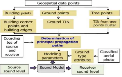
The flow chart shown in Figure 1 demonstrates the steps employed for determination of terrain parameters and their consequent use for sound modelling. LIDAR data points are classified to building, ground and tree points. Building corner and edges of roof are extracted from building class manually and are used subsequently to determine the possible diffracting paths for a combination of source and receiver using cutting plane technique. The ground and tree points are triangulated separately and processed further to derive reflective paths or through-tree paths for the source and receiver pair. Aerial Photograph is used to associate ground points with the ground type information for determining reflection coefficient for the ground. Different terrain parameters required for sound modelling such as distance between source and receiver, length of path difference for diffraction, reflection coefficient, tree absorption length etc are determined, using simple geometric relationships, along different principal paths identified above. Detail terrain parameters, derived for a source and receiver multiple receivers or multiple sources multiple receivers cases.
Figure 1. Flow chart showing extraction of terrain parameters and sound modelling
3.1 Data preparation:
LIDAR data employed in this work were collected over IIT Kanpur, India with an approximate density of 1 point/m2. LIDAR data are classified as building, ground and tree classes using commercial software Terrascan. Classified point clusters of different classes are used to extract principal paths and terrain parameters. Ground and tree point clusters are triangulated and used to generate reflective or through-tree paths. Satellite image with 5 m resolution is used as spectral information, in place of Aerial Photograph. Satellite imagery is registered with LIDAR data and classified to provide ground type information to LIDAR points. Details of each step in algorithm are described below.
3.2 Determination of direct transmission path and decision on possibilities of other paths:
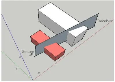
In order to determine various principal paths a plane perpendicular to X-Y plane (ground plane) is considered which contains source and receiver locations (Figure 2). It is ascertained first whether this plane (referred as cutting plane) intersects any of the building walls or obstructions in between the source and receiver locations. Points of intersection are ISPRS Annals of the Photogrammetry, Remote Sensing and Spatial Information Sciences, Volume I-4, 2012
determined from equation of cutting plane and equations of lines corresponding to edges of buildings or obstructions. In case it finds no building or obstruction in between the source and receiver the sound will transmit through two paths, i.e., direct and ground reflected. In this scenario additional path(s) can also exist that contribute sounds to receiver location, if there exists natural reflector such as boundary wall, building etc close to the source or receiver, which can specularly reflect sound to receiver. The principal path for direct transmission is the straight line connecting source to receiver. The technique for determining reflecting path(s) is described in section 3.5. In case any building wall etc. gets intersected by the above cutting plane, diffracting paths over the top and around the sides of buildings are required to be determined along with reflecting paths. The path through a tree is determined if any of the above paths intersect a tree to reach the receiver. The techniques for determining diffracting, reflecting and through-tree paths are explained in sections 3.3 to 3.6.
3.3 Determining diffracting path over roof top:
In order to determine diffracting path over roof top, the points of intersection between cutting plane (as in 3.2) and building roof edges are located (Figures 2 and 3). These points form a set of all potential diffracting points over the top of intermediate buildings. The effective points of diffraction, in this case, are determined from this set of potential points (Figure 3). First, the highest diffracting point is located. Sound emitted from source reaches the receiver through this highest diffracting point following the shortest path. However, if the direct path connecting source to the highest diffracting point also gets obstructed by any other roof top, the diffracting points associated with intercepting roof edges are identified. The nearest of these diffracting point (from the source location) is considered to be the first diffracting point. The algorithm runs similarly till it reaches the highest diffracting point (in Figure 4 since the direct path is not intercepted by any roof edge, the tallest diffracting point c becomes the first diffracting point). After reaching the highest diffracting point the algorithm tries to reach the receiver directly. If it gets obstructed by any potential diffracting point, the nearest-to-tallest-diffracting-point is considered to be the next diffracting point (in Figure 4, d becomes the next diffracting point after c). It runs iteratively with above rule from this diffracting point till it reaches the receiver location. When all the effective diffracting points are located, the principal path is the path which joins these points (Figure 5).
Figure 2. Cutting plane technique of determining potential points for diffraction over top (cutting plane X-Y plane)
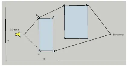
Figure 3. Potential diffracting points over top (a, b, c, d are potential diffracting points determined by intersection of cutting
plane and building roof edges)
Figure 4. Determination of successive diffracting points. Here a, b, c, d are potential diffracting points of which c is the highest.
The line connecting source to highest diffracting point is not obstructed by any other vertical edge hence c becomes the first
diffracting point
Figure 5. Final diffracting path over top. It is determined from effective diffracting points between source and receiver
3.4 Determination of diffracting path around sides:
Similar to the path over top, the paths around sides of building or wall or obstruction are determined using another cutting plane. A plane perpendicular to X-Z plane and passing through and bounded by the source and receiver is considered as cutting plane (Figure 6). The edges of buildings/walls that are intersected by the plane are determined (Figure 7).
Figure 6. Cutting plane technique to determine potential points of diffraction around sides (cutting plane X-Z plane)
Figure 7. Potential points of diffraction around sides
Figure 8. Potential points and edges (projected to X-Y) to be used for determining effective diffracting points
around sides
Figure 9. Determination of principal paths around sides The potential points and associated edges are then projected to X-Y plane (Figure 8).These edges are then used to determine the effective points of diffraction around sides. The edge nearest to the source location is selected first. Two terminus of this edge (a and b in Figure 9) are determined to be the first diffracting points for the two separate side paths. Continuing from these points the algorithm tries to determine the respective next point of diffraction. In order to determine this, algorithm considers
that sound will reach the receiver directly. However, if it gets obstructed by building edge(s), the existence of other intermediate diffracting point(s) is confirmed. The successive diffracting point for respective side paths are then determined based on multiple criteria decision rule. This rule includes the guidelines such as (i) the diffracting path around side should not cross any edge, but it can diffract around edge (ii) diffracting path around side should not choose any of the edge selected earlier (iii) in case of multiple possibilities, the edge should be decided making the shortest transmission path. The algorithm runs iteratively determining successive diffracting points before reaching the receiver. This algorithm determines two shortest paths around sides (as shown in Figure 9).
3.5 Determination of reflection path for ground or wall:
Ground and building walls are evaluated if they act as reflector of sound. Ground LiDAR points and the points representing the side walls of building are triangulated separately. Each triangle in Triangulated Irregular Network (TIN), closer to receiver and source, is considered as a potential reflector and tested for the near specular reflection criteria (Figures 10 and 11). A plane is constructed containing the centroid of triangle, source and the receiver. The normal to the plane and respective triangle are evaluated to know, (i) if the plane and triangle are orthogonal and (ii) if the incidence and reflection angles are equal thus satisfying the specular reflection criterion. Having tested all potential triangles the one satisfying the criteria best is chosen as the reflecting point of sound. The classified surface type information (ground type from Aerial Photograph) is used to determine the reflection coefficient of the reflecting triangle (Bies, et. al., 2003).
Figure 10. Determination of ground reflecting point.
(Determination of TIN triangle orthogonal to source-receiver vertical plane and following specular reflection criteria)
Figure 11. Determination of reflection from wall ISPRS Annals of the Photogrammetry, Remote Sensing and Spatial Information Sciences, Volume I-4, 2012
3.6 Determination of through-tree path:
To determine the through-tree path, clusters are formed using K-mean algorithm amongst all the points classified as tree or vegetation. Tetrahedrons are generated for all points that belong to a cluster. The reflecting and diffracting paths, as determined in the above steps, are checked if these are intercepted by tree clusters. The intercepting faces (triangles in tetrahedrons), located farthest from each other for a cluster, are considered as the extent of principal path that is passing through a tree and leads to absorption (Figure 12). This is repeated for all the clusters intercepting the path. Finally all the intercepting lengths are added to determine total length of path for tree absorption of sound.
Figure 12. Determination of through-tree length (path length intercepted by tree cluster)
3.7 Determination of terrain parameters and sound modelling:
Principal paths determined in sections 3.2-3.6 are used to obtain different terrain parameters i.e., different distances, path difference, angle of reflection etc (as listed in the first paragraph f section 1). Simple geometric relationships are used for determining the above terrain parameters. For example (i) the distance between two points with known coordinates is used for determining path length for direct transmission path and other indirect transmission paths between source and receiver (ii) the angle between intersecting lines in a plane is used for determining ground or wall reflecting angle. Above terrain parameters are incorporated inside semi-empirical sound model for prediction of sound at receiver location. Discussion on semi-empirical sound model is beyond the scope of this paper. However, the following experiment is used to validate the accuracy of sound prediction, thus indirectly validating the technique of principal path identification, which is the main focus of this paper, using the extracted terrain parameters and sound model.
4. EXPERIMENTAL VALIDATION AND GENERATION OF NOISE MAP
The experiment on sound propagation modelling is conducted in an outdoor environment for a field having buildings, trees and different ground types at IIT Kanpur. LIDAR data and satellite image are available for this site (Figure 13). Tonal sounds of four frequencies (250, 500, 1000, 4000 Hz) and known sound pressure levels (85dB-122dB) are generated at a fixed location in the field. The transmitted sound is measured at 210 different locations in 3D space using sound pressure level meter. Sound pressure level at these 210 points is also modelled using the sound model employed in this work. The measured sound pressure levels are compared against modelled sound pressure levels. The differences are analyzed statistically and against the reported literature (Bies, et. al., 2003) to determine
efficacy of the proposed technique for sound propagation modelling (Table 1). The table shows that the predictions differ from measurement by 7.1 to 9.6 dB as against deviation of 10-20 dB as reported in literature (Bies, et. al., 10-2003). The comparison is made on the basis of tonal sounds i.e., sounds of individual frequency.
Table 1. Table showing statistics of difference in measured and modelled sound pressure levels for four frequencies. Mean(Stdv) are computed for differences irrespective of their sign. Difference reported in literature is given in the last column (Bies, et. al., 2003).
The developed technique is used to generate the sound level map (the term “noise map” will be used henceforth instead of
“sound level map” as this is more commonly used) for a part of
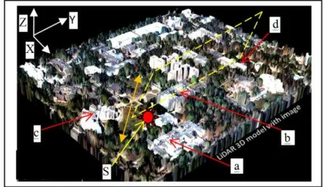
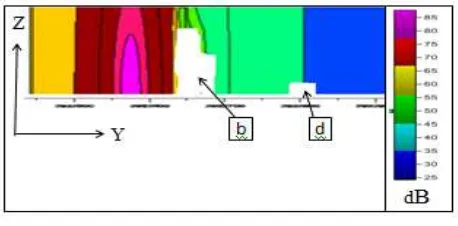
academic area at IIT Kanpur. A hypothetical sound source (omni-directional tonal sound of 250 Hz at 100 dB) marked as S in Figure 13 is considered. Sound levels are predicted in dB for all points on the LIDAR DSM and displayed corresponding to their X, Y locations in Figure 14 using the shown colour scale. In can be seen from Figures 13 and 14 that higher level of sound pressure is found in the unobstructed direction (marked by double sided arrow). Similarly, the diffraction is causing significant attenuation in sound pressure levels around the buildings (as noticed at a, b, c and d). To understand the spread of sound in the space above DSM up to a height of 20 m additional sound pressure levels are modelled along a section (parallel to Y-Z plane as shown by yellow dashed rectangle in Figure 13). The resulting sound pressure levels are shown in Figure 15. Buildings b and d are also shown in the section. The buildings b and d in Figure 15 are shown as white as no sound transmits inside the building and thus no prediction is made.
Figure 13 LIDAR 3D model of IIT Kanpur academic area. a, b, c, d are positions of buildings and S the position of sound source. Double sided yellow arrow indicates major unobstructed
propagation direction. ISPRS Annals of the Photogrammetry, Remote Sensing and Spatial Information Sciences, Volume I-4, 2012
Figure 14. Noise map of academic area of IIT Kanpur. Modelled sound pressure levels (dB) are displayed with colours
for all points in DSM due to sound generated by the source placed at S. Points a, b, c, d are positions of buildings. The
double sided yellow arrow indicates major unobstructed propagation direction.
Figure 15. A section along Y-Z plane is drawn from DSM to a height of 20m. Modelled sound pressure levels are displayed
with colour.
5. CONCLUSION
A technique, with the aim to incorporate terrain parameters for sound propagation modelling, is developed to identify principal paths of sound transmission using high resolution LIDAR data and Aerial Photograph. The paper used a mixed approach to determine the principal paths of sound propagation. The cutting plane technique developed provides an accurate and efficient way to locate principal paths through top and sides of a building or a group of buildings. A further technique has been developed to locate the point of reflection between source and receiver. Classified Aerial Photograph is used to determine the ground type information for fixing the reflection coefficient. The transmission length through trees is computed using the tetrangulated cluster of tree LiDAR points. Extracted terrain parameters are incorporated inside the sound model for sound prediction. The developed technique is validated using an intensive field experiment. The results show that the developed technique predicted sound pressure levels better to those reported in literature with differences ranging from 7.1 to 9.6 dB for tonal sounds of different frequencies. Further, the technique can be utilized for generating noise map (sound pressure level map) of an area, as has been demonstrated through the development of 3D noise map for the study site.
5.1 References and selected bibliography
Bies, A., D., and Hansen, H., C., 2003. Engineering noise control, Spon Press, Great Britain, pp. 92-400.
David, C., Jenny, S., & Bill, O., 2002. “Assessment of data sources and available modeling techniques-are they good enough for comprehensive coverage by computer noise
mapping”.
http://www.cerc.co.uk/services/Noise%20Mapping%20CERC% 20IofA%20Feb2002.pdf (accessed 12 May 2006)
Environmental Noise Directive, European Parliament and Council, 2002, Directive 2002/49/EC of 25 June 2002.http://en.wikipedia.org/wiki/Noise_map#Directive_2002.2 F49.2FEC (accessed 24 April 2011).
Kurze, U., J., 1973. Noise reduction by barriers. Journal of Acoustic Society of America, 55(3), pp. 504-518.
Maekawa, Z., 1968. Noise reduction by screens., Applied Acoustics, 1, pp. 157–173.
Renzo Tonin, 2005., “Modeling and predicting environmental noise”. http://www.rtagroup.com.au/pdfs/22.pdf (accessed 15
Nov. 2006).
Rossing, D. T., 2007. Handbook of Acoustics, Springer, NY, USA, pp. 113-147.
RTA group, 1989., ENM-Environmental Noise Model
“Program Specification”. http://www.rtagroup.com.au/ enm/environmental_noise_model.html (accessed 7 Dec. 2007). Ibrahim, S., 2003, Feature extraction and 3D city modeling using airborne LIDAR and high resolution digital ortho photos a comparative study, Master Project, University of Texas at Dallas.
Lohani, B., and Singh, R.,2007, Development of a Hough Transform based algorithm for extraction of buildings from actual and simulated LIDAR data, Proceedings of Map World Forum 2007, Hyderabad
Tse, R. O. C. Gold, C. M., and Kidner, D. B.; 2004, Building reconstruction using LIDAR data. ISPRS Workshop on Updating Geo-spatial Databases with Imagery & The 5th ISPRS Workshop on DMGISs