Using variance analysis of multitemporal MODIS images for rice field mapping in Bali Province, Indonesia.

(1)

On: 12 July 2013, At : 06: 39 Publisher : Taylor & Francis

I nfor m a Lt d Regist er ed in England and Wales Regist er ed Num ber : 1072954 Regist er ed office: Mor t im er House, 37- 41 Mor t im er St r eet , London W1T 3JH, UK

International Journal of Remote

Sensing

Publ icat ion det ail s, incl uding inst ruct ions f or aut hors and subscript ion inf ormat ion:

ht t p: / / www. t andf onl ine. com/ l oi/ t res20

Using variance analysis of

multitemporal MODIS images for

rice field mapping in Bali Province,

Indonesia

I Wayan Nuarsa a , Fumihiko Nishio b , Chiharu Hongo b & I Gede Mahardika a

a

Facul t y of Agricul t ure, Udayana Universit y, Denpasar, 80361, Indonesia

b

Cent re f or Environment al Remot e Sensing, Chiba Universit y, Chiba, 263‐8522, Japan

Publ ished onl ine: 01 Mar 2012.

To cite this article: I Wayan Nuarsa , Fumihiko Nishio , Chiharu Hongo & I Gede Mahardika (2012) Using variance anal ysis of mul t it emporal MODIS images f or rice f iel d mapping in Bal i Province, Indonesia, Int ernat ional Journal of Remot e Sensing, 33: 17, 5402-5417, DOI: 10. 1080/ 01431161. 2012. 661091

To link to this article: ht t p: / / dx. doi. org/ 10. 1080/ 01431161. 2012. 661091

PLEASE SCROLL DOWN FOR ARTI CLE

Taylor & Francis m akes ever y effor t t o ensur e t he accuracy of all t he infor m at ion ( t he “ Cont ent ” ) cont ained in t he publicat ions on our plat for m . How ever, Taylor & Francis, our agent s, and our licensor s m ake no r epr esent at ions or war rant ies w hat soever as t o t he accuracy, com plet eness, or suit abilit y for any pur pose of t he Cont ent . Any opinions and view s expr essed in t his publicat ion ar e t he opinions and view s of t he aut hor s, and ar e not t he view s of or endor sed by Taylor & Francis. The accuracy of t he Cont ent should not be r elied upon and should be independent ly ver ified w it h pr im ar y sour ces of infor m at ion. Taylor and Francis shall not be liable for any losses, act ions, claim s, pr oceedings, dem ands, cost s, expenses, dam ages, and ot her liabilit ies w hat soever or how soever caused ar ising dir ect ly or indir ect ly in connect ion w it h, in r elat ion t o or ar ising out of t he use of t he Cont ent .

(2)

Condit ions of access and use can be found at ht t p: / / w w w.t andfonline.com / page/ t er m s-and- condit ions

(3)

Vol. 33, No. 17, 10 September 2012, 5402–5417

Using variance analysis of multitemporal MODIS images for rice field

mapping in Bali Province, Indonesia

I WAYAN NUARSA*†, FUMIHIKO NISHIO‡, CHIHARU HONGO‡ and I GEDE MAHARDIKA†

†Faculty of Agriculture, Udayana University, Denpasar 80361, Indonesia ‡Centre for Environmental Remote Sensing, Chiba University, Chiba 263-8522, Japan

(Received 18 December 2009; in final form 10 December 2011)

Existing methods for rice field classification have some limitations due to the large variety of land covers attributed to rice fields. This study used temporal vari-ance analysis of daily Moderate Resolution Imaging Spectroradiometer (MODIS) satellite images to discriminate rice fields from other land uses. The classification result was then compared with the reference data. Regression analysis showed that regency and district comparisons produced coefficients of determination (R2₎ of 0.97490 and 0.92298, whereas the root mean square errors (RMSEs) were 1570.70 and 551.36 ha, respectively. The overall accuracy of the method in this study was 87.91%, with commission and omission errors of 35.45% and 17.68%, respectively. Kappa analysis showed strong agreement between the results of the analysis of the MODIS data using the method developed in this study and the reference data, with a kappa coefficient value of 0.8371. The results of this study indicated that the algorithm for variance analysis of multitemporal MODIS images could potentially be applied for rice field mapping.

1. Introduction

Rice is one of the most important agriculture crops in many Asian countries, and it is a primary food source for more than three billion people worldwide (Khush 2005, Yanget al. 2008). Mapping the distribution of rice fields is important not only for food security but also for management of water resources and estimations of trace gas emissions (Matthews et al. 2000, Xiao et al. 2005). Therefore, more accurate data related to the total rice field area, its distribution and its changes over time are essential.

Satellite remote sensing has been widely applied and is recognized as a powerful and effective tool for identifying agriculture crops (Bachelet 1995, Le Toan et al. 1997, Fang 1998, Fanget al. 1998, Liewet al. 1998, Okamoto and Kawashima 1999, Niel et al. 2003, Bouvet et al. 2009, Pan et al. 2010). This process primarily uses the spectral information provided by remotely sensed data to discriminate between perceived groupings of vegetative cover on the ground (Niel and McVicar 2001). Although spectral dimension is the basis of remote-sensing-based class discrimination, temporal and spatial resolutions play very important roles in classification accuracy.

*Corresponding author. Email: nuarsa@ymail.com

International Journal of Remote Sensing

http://dx.doi.org/10.1080/01431161.2012.661091

(4)

Discrimination of crops is usually performed with ‘supervised’ or ‘unsupervised’ clas-sifiers. The basic difference between these types of classification is the process by which the spectral characteristics of the different groupings are defined (Atkinson and Lewis 2000). Common classification algorithms include the maximum likelihood, minimum distance to mean and parallelepiped (Jensen 1986).

The high temporal remote-sensing data now available from various platforms offer an opportunity to exploit the temporal dimension for crop classification. The use of data sets of high temporal vegetation indices (VIs) for crop studies calls for new classi-fication approaches. The Moderate Resolution Imaging Spectroradiometer (MODIS) is one of the satellite sensors that provide daily revisit times. A MODIS image has a high ability to discriminate agricultural crops (Boschettiet al. 2009, Tingting and Chuang 2010).

Agricultural rice fields have a large variety of land covers, which can range from waterbodies just before rice transplanting to mixed water, vegetation or bare soil just after harvesting time. The range of land covers and the complex relationships between ecological factors and land-cover distribution cannot be accurately expressed through deterministic decision rules (Hutchinson 1982, Mas and Ramírez 1996). Alternatively, the large variety of rice field land covers compared with other land uses can be advantageous in distinguishing rice fields from other land uses.

The objectives of this study are to develop a new algorithm for rice field classifi-cation using temporal variance analysis and quantitatively compare the classificlassifi-cation result using the new method with the existing method using reference data.

2. Study area, data and method

2.1 Background and study area

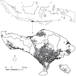
The study area is located in the Bali Province of Indonesia and is centred at latitude 8◦₄₀′₀₀′′_{S and longitude 115}◦₁₉′₀₀′′ _{E (figure 1). Besides being a popular}

interna-tional tourism destination, Bali Island, although relatively small, is also historically one of the prime rice-producing areas in Indonesia. Approximately 0.5 million tons (1.6% of Indonesia’s rice production) is contributed by Bali Province. Agriculture rice fields in Bali consist of irrigated fields and non-irrigated fields. The water sources for the irrigated rice fields are rivers, whereas the water for non-irrigated rice fields comes from rainfall. Annually, both irrigated and non-irrigated rice field lands are not only used for rice paddies but also for seasonal crops, such as corn, soya beans and nuts. However, the type of seasonal plant grown from year to year is usually similar from one place to another. In humid tropical regions, such as in the study area, rice plants can be planted at any time. However, planting is influenced by water availabil-ity. Therefore, for irrigated land, rice planting alternates between regions, whereas in non-irrigated land, rice planting occurs in the rainy season. Farmers usually plant the rice two or three times per year, and use the remaining time for other seasonal crops (Food Crops Agriculture Department 2006). The crop growth duration is approxi-mately 3 months, with a production of around 5 tons per hectare. The total rice acreage of the study region as reported for the year of 2008 is 107 437.50 ha (table 1).

2.2 MODIS images

This study used daily MODIS 1b level images (calibrated radiances), with a spatial resolution of 250 m (MOD02QKM). The images can be downloaded free from the

(5)

N

10 0 20 km

Figure 1. Map of the study area. Bali province consists of nine regencies. Black colour indicates the distribution of rice fields.

Table 1. Reported total rice acreage in Bali by regency (National Land Agency 2008).

Regency Total area (ha) Rice field area (ha) Rice field percentage

Badung 39 450.00 12 887.50 32.67

Bangli 52 718.75 3 537.50 6.71

Buleleng 131 925.00 13 606.25 10.31

Denpasar 12 506.25 4 181.25 33.43

Gianyar 36 431.25 16 800.00 46.11

Jembrana 85 418.75 9 462.50 11.08

Karangasem 83 662.50 11 418.75 13.65

Klungkung 31 231.25 6 462.50 20.69

Tabanan 84 818.75 29 081.25 34.29

Total 558 162.50 107 437.50 100.00

NASA website (http://ladsweb.nascom.nasa.gov/data/search.html). This data product offers the best available spatial resolution among all other MODIS products. A coarser spatial resolution will increase the possibility of mixed land coverage occurring in one pixel, decreasing the accuracy of the classification result (Strahleret al. 2006).

(6)

In addition, at this level of MODIS imaging, there are several images for each acqui-sition date taken at different times. This level of imaging can increase the possibility of a clear image without clouds, which has become a big challenge in optical remote sensing.

Two spectral band data, viz. red (620–670 nm) and near-infrared (NIR, 841–875 nm), were used for this. We collected the MODIS images at different acqui-sition dates and times over a 2 year period (2008 and 2009). Data of 2009 were used to develop the model, and that of 2008 were utilized to validate the model because the reference land-use map was dated 2008. Cloud cover is not intense in the rice region of the study area, as clouds more frequently occur at higher elevations. However, to produce a cloud-free image, cloud masks were generated using two-band data for each acquisition date. Each cloudy pixel was replaced with a clear pixel from another image obtained within 14 days of the original. A total of 52 composite images were used in this study.

2.3 Calculation of VI

Three VIs were selected – the normalized difference VI (NDVI), ratio VI (RVI) and soil-adjusted VI (SAVI). We used the radiance value of the MODIS images for each 14-day composite. The equations for these VIs are as follows:

NDVI= Rnir−Rr Rnir+Rr

, (1)

RVI= Rnir Rr

, (2)

SAVI=(1+L)(Rnir−Rr) Rnir+Rr+L

, (3)

where Rnir is the reflectance in the MODIS NIR band (841–876 nm), Rr is the

reflectance in the red band (620–670 nm) andL is a constant (related to the slope of the soil line in a feature-space plot) that is usually set equal to 0.5.

Although NDVI is correlated to the leaf area index (LAI) of rice fields (Xiaoet al. 2002), it has some limitations, including saturation under closed canopy and soil back-ground (Hueteet al. 2002, Xiaoet al. 2003). The SAVI can minimize soil brightness influences from spectral VIs involving red and NIR wavelengths (Huete 1988). On the other hand, the RVI is a good indicator of agriculture crop growth for the entire growth cycle (Gupta 1993).

The advantages of using a VI compared with a single band is the ability to reduce the spectral data to a single number that is related to physical characteristics of the vegetation (e.g. leaf area, biomass, productivity, photosynthetic activity or percentage cover) (Huete 1988, Baret and Guyot 1991). At the same time, we can minimize the effect of internal (e.g. canopy geometry and leaf and soil properties) and external fac-tors (e.g. sun–target–sensor angles and atmospheric conditions at the time of image acquisition) on the spectral data (Huete and Warrick 1990, Baret and Guyot 1991, Huete and Escadafal 1991).

(7)

2.4 Algorithm for rice field mapping

The main difference in agriculture rice field characteristics compared with other land uses is the variation of land cover due to many types of vegetation planted in rice field areas. In irrigated rice fields, when the rice is planted, its land cover can vary from flooded at the beginning of transplanting to mixed between water and vegetation in the first month, almost full vegetation in the second and third month and bare area just after harvesting time. The variation in land cover can be greater when the rice field area is planted with other seasonal crops. Similar cases also occur in non-irrigated rice fields, which have a significant difference in land cover between the rainy season (rice season) and dry season (other seasonal crops). On the other hand, other land uses, such as settlement, forest and water, generally have similar land covers within a cer-tain period. This situation will affect the reflectance value at cercer-tain times. Rice fields will have a fluctuating reflectance value, whereas other land uses will have relatively stable values. Based on these phenomena, temporal variance analysis is used to distin-guish between rice field areas and other land uses. The hypothesis proposed is that the radiance variance of the rice field will be much higher than that of other land uses.

Temporal VI data were used to generate the temporal variance map. A field survey was carried out to confirm the location of the training area on the image, besides using the available land-use or land-cover map. The training classes covered under field survey were irrigated rice field, non-irrigated rice, mixed forest, settlement, lake water, mixed garden, shrub, dry land, mangrove and bare land. These 10 training classes were used to determine their variance in a year in each of the three VI image data sets. From the VI variance map, we calculated the mean and standard deviation of variance for the 10 objects. The formulae for the variance, mean of variance and standard deviation of variance were calculated using the following equations:

variance= 1

of images (which is equal to 26 in this study),

mean=1

wherexiis the variance value of a pixel for the training areai,x¯is the mean of variance

andnis the number of pixels in the training area.

From the three VIs evaluated, the VI with the highest difference in the mean vari-ance was selected as the best VI for distinguishing rice field and other land uses. Threshold values were required for rice field mapping. The pixel ranges within the threshold were mapped as rice fields with the following equation:

Vmean−(nS)<x<Vmean +(nS), (7)

(8)

whereVmean,S,nandxare the average of the rice field variance, the standard

devia-tion of the rice field variance, the maximum distance from the standard deviadevia-tion and the variance average of the MODIS image that will be mapped as a rice field class, respectively.

2.5 Quantitative evaluation of the classification result

The quantitative evaluation was performed by comparing the classification result with the existing land-use maps released by the National Land Agency. To determine the accuracy of the classification method developed in this study, we used two evaluation methods. First, we used a regression method using the area obtained from the anal-ysis result and the reference data for the rice field as the dependent and independent variables, respectively. The coefficient of determination (R2_{) and the root mean square}

error (RMSE) were the two statistical parameters evaluated in this study. The regres-sion methods were applied at the regency and district level using 9 and 52 samples, respectively, based on the number of regencies and districts in the study area. TheR2

and RMSE were calculated as follows:

R2= y− ˆy 2

y− ¯ˆy2

, (8)

where R2_, _y_, _y_ˆ _and_y_¯ˆ _{are the coefficient of determination, the measured value, the}

estimated value and the mean of the estimated values, respectively, and

RMSE=

where RMSE,yˆi,yiandnare the root mean square error, the estimated value ofifrom

the analysis result, the reference value ofiand the number of data, respectively. The second evaluation method used kappa analysis (Congalton and Green 1999). The kappa analysis determined accuracy assessments and the level of agreement between the remotely sensed classification and the reference data. The first step of kappa analysis is to create an error matrix for all the examined methods. In this study, only two classes were used: rice field and non-rice field. From the error matrix, we can calculate the commission error, omission error and overall accuracy as follows:

commission error=total number of pixels in non-rice fields classified as rice field

total number of pixels classified as rice field ×100, (10)

omission error= total number of rice field pixels not classified as rice field

total number of actual rice field pixels ×100,

(11)

overall accuracy= total number of correctly classified pixels

total number of pixels in sample ×100. (12)

(9)

The next step of the kappa analysis is to calculate the estimated kappa coefficient and

whereKˆ is the estimated kappa coefficient, n is the number of sample tests,iis the sample row,j is the sample column and kis the number of ‘rows×columns’. The formula for the kappa variance is

varˆ Kˆ= 1

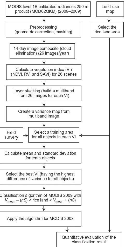
The estimated kappa values range from 0 to 1, although they can be negative and range from –1 to 1. However, because there should be a positive correlation between the remotely sensed classification and the reference data, positive kappa values are expected. A perfect classification would produce a kappa value of 1 and kappa vari-ance of 0. Typically, values greater than 0.80 (i.e. 80%) represent strong agreement between the remotely sensed classification and the reference data, whereas values between 0.4 and 0.8 represent moderate agreement. Anything below 0.4 is indicative of poor agreement (Congaltonet al. 1983). Schematically, the research procedure is shown in figure 2.

3. Results and discussion

3.1 Temporal variability of the VI of land uses

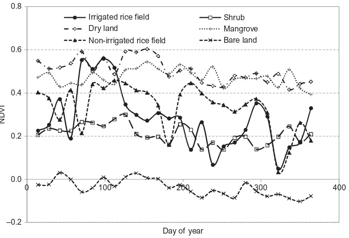
The VI of land uses varied in the study area during 2009. The highest variabil-ity appeared in the irrigated rice fields, followed by the non-irrigated rice fields. The other land uses, such as settlement, mixed garden, mixed forest, lake water, dry land, shrub, mangrove and bare land, had a relatively stable VI over the year. The NDVI of the irrigated rice field was high at certain times and over-lapped with mixed forest, mixed garden, dry land and mangrove. However, the value

(10)

MODIS level 1B calibrated radiances 250 m product (MOD02QKM) (2008–2009)

Preprocessing (geometric correction, masking)

Land-use map

Select the rice land area

14-day image composite (cloud elimination) (26 images/year)

Calculate vegetation index (VI) (NDVI, RVI and SAVI) for 26 scenes

Layer stacking (build a multiband from 26 images for each VI)

Create a variance map from multiband image

Field survery

Select a training area for all objects in each VI

Calculate mean and standard deviation for tenth objects

Select the best VI (having the highest difference of variance for all objects)

Classification algorithm of MODIS 2009 with Vmean – (nS) < rice land < Vmean + (nS)

Apply the algorithm for MODIS 2008

Quantitative evaluation of the classification result

Figure 2. Flow chart of the research procedure.Vmean,Sandnare the average of the rice field variance, the standard deviation of the rice field variance and the maximum distance from the standard deviation, respectively.

was low at other times and was similar to the values for settlement and shrub (figures 3 and 4). The non-irrigated rice field also had a similar tendency, although NDVI values were not as high as that observed with the irrigated rice field. The high fluctuations in the VI of irrigated and non-irrigated rice fields were due to the high variation in their land covers. When the areas were being planted with rice plants

(11)

–0.6 –0.4 –0.2 0.0

ND

VI

Day of year Irrigated rice field

Settlement Mixed garden

Mixed forest Lake water

Non-irrigated rice field

0 100 200 300 400

0.2 0.4 0.6 0.8

Figure 3. The NDVI temporal variability of irrigated rice fields, non-irrigated rice fields, settlement, mixed garden, mixed forest and lake water from 1 January to 31 December.

–0.2

ND

VI

Day of year Irrigated rice field

Dry land

Non-irrigated rice field

Shrub Mangrove Bare land

0 100 200 300 400

0.0 0.2 0.4 0.6 0.8

Figure 4. The NDVI temporal variability of irrigated rice fields, non-irrigated rice fields, dry land, shrub, mangrove and bare land from 1 January to 31 December.

(12)

or other seasonal crops, the VI was similar to that of mixed forest, mixed garden, mangrove or shrubs. However, if no crops were planted, the land cover resembled settlement or bare land.

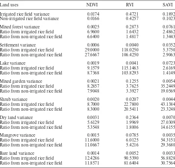
The irrigated rice field had the highest average variance of 0.0174, 0.4721 and 0.1892 for the NDVI, RVI and SAVI, respectively. The non-irrigated rice field was next, with index values of 0.0166, 0.0989 and 0.1023 for the NDVI, RVI and SAVI, respec-tively. The lowest average variance occurred for settlement, with values of 0.0006 and 0.0040 for the NDVI and RVI, respectively. The bare land had the lowest aver-age variance for the RVI with a value of 0.0033. Compared with other land uses, the average variance of the irrigated rice fields was higher, ranging from 5.6129 to 29.0000 times higher for the NDVI, 1.6432–118.0250 times higher for the RVI and 2.4862–56.8828 times higher for the SAVI. For the non-irrigated rice fields, the aver-age variances were 5.3548–27.6667 higher for the NDVI, 1.4817–106.4250 higher for the RVI and 1.3443–30.7564 higher for the SAVI (table 2).

The RVI can easily be used to distinguish both irrigated and non-irrigated rice fields from other land uses, such as settlement, lake water, shrub and bare land. However, it would be difficult to use the RVI to distinguish irrigated and non-irrigated rice fields

Table 2. Mean of irrigated and non-irrigated rice field variance compared with other land uses.

Land uses NDVI RVI SAVI

Irrigated rice field variance 0.0174 0.4721 0.1892

Non-irrigated rice field variance 0.0166 0.4257 0.1023

Mixed forest variance 0.0025 0.2873 0.0761

Ratio from irrigated rice field 6.9600 1.6432 2.4862

Ratio from non-irrigated rice field 6.6400 1.4817 1.3443

Settlement variance 0.0006 0.0040 0.0352

Lake variance 0.0019 0.0041 0.0723

Mixed garden variance 0.0021 0.1255 0.0054

Shrub variance 0.0020 0.0207 0.0044

Dry land variance 0.0031 0.2364 0.0070

Mangrove variance 0.0015 0.0785 0.0035

Bare land variance 0.0014 0.0052 0.0033

(13)

from mixed forest and dry land because the difference in their variances is small. A similar case occurred for the SAVI. The SAVI can easily separate irrigated and non-irrigated rice fields from mixed garden, shrub, dry land, mangrove and bare land. However, it was very difficult to differentiate mixed forest and lake water from non-irrigated rice fields using SAVI. On the other hand, the NDVI can easily distinguish both irrigated and non-irrigated rice fields from other land uses due to the minimum value of their difference variances, which were 5.6129 and 5.3548 for irrigated and non-irrigated rice fields, respectively. Therefore, the NDVI was selected for rice field mapping.

3.2 Classification of rice fields

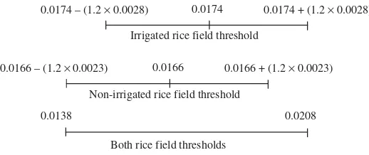
To apply the NDVI variance for rice field mapping, a threshold value was determined. According to equation (7), the mean and standard deviation of the rice field NDVI variance will be used as the threshold value. The mean and standard deviation were 0.0174 and 0.0028 for irrigated rice fields and 0.0166 and 0.0023 for non-irrigated rice fields, respectively (table 3).

The differences in the mean and standard deviations of the irrigated and non-irrigated rice field variance were not large. Therefore, using non-irrigated and non-non-irrigated rice fields as separate classes proved difficult because of some overlapping values. Therefore, both types of rice field were mapped as one class. Based on the analysis results, using a value ofnof 1.2 in equation (7) provided the best result. Therefore, the threshold value of both types of rice field is as follows:

0.0174 + (1.2 × 0.0028) 0.0174 – (1.2 × 0.0028) 0.0174

Irrigated rice field threshold

0.0166 + (1.2 × 0.0023) 0.0166 – (1.2 × 0.0023) 0.0166

Non-irrigated rice field threshold

0.0208 0.0138

Both rice field thresholds

The pixels having a temporal variance between 0.0138 and 0.0208 were classified as a rice field. Although irrigated and non-irrigated rice fields had the highest mean tempo-ral variance, we did not use a threshold value greater than or equal to 0.0138 because of the cloud effect in the MODIS images. Although a 14 day composite was created to replace cloudy images with clearer images, it is very difficult to remove all of the clouds from MODIS images, especially in tropical areas. Thin clouds greatly affect the reflectance and the VIs and increase the temporal variance of the pixel. Therefore, to avoid classifying a cloudy pixel as a rice field, we used the maximum threshold. In this

Table 3. Mean and standard deviation of the variance for irrigated and non-irrigated rice fields.

Rice field Mean Standard deviation

Irrigated rice field variance 0.0174 0.0028

Non-irrigated rice field variance 0.0166 0.0023

(14)

study, we did not classify all of the land uses found in the study area because only rice fields had a high variability in the temporal variance. Other land uses, such as mixed garden, shrub and mixed forest, had similar variances and would become a single class if the algorithm was applied. The same is true for lake water, mangrove and bare land (table 2).

The change in the land cover of rice fields from the initial flooding of the fields to harvesting takes place over a short period of time. This change will produce large differences in spectral values and in the rice field indices over that time. The high degree of variation in the land cover of the rice field could be used to obtain more effective separation of rice fields from other land uses, using the variance analysis presented here.

The results of the rice field classification using the algorithm developed in this study are shown in figure 5. Compared with the reference data (figure 5(a)), the rice field map produced from our analysis (figure 5(b)) was visually similar to the reference.

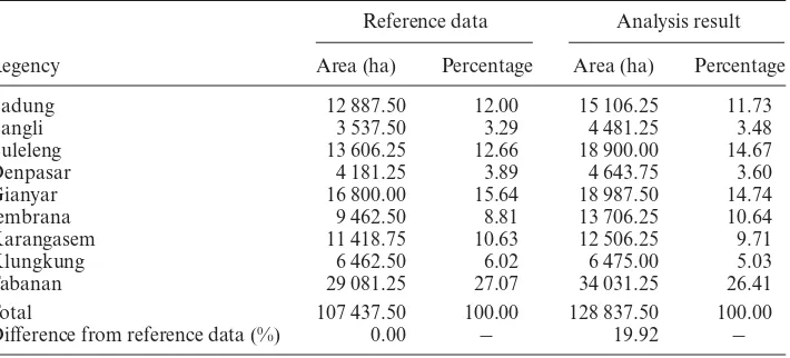
Table 4 shows a quantitative comparison between the algorithm used in this study and the reference data. The analysis showed 19.92% deviation compared with the reference data.

(a₎ ₍b₎

Figure 5. Rice field maps derived from this analysis (b) compared with reference data (a). Black colour on the map shows the distribution of rice fields.

Table 4. Comparison of rice area derived from this analysis with the reference data at the regency level.

Reference data Analysis result

Regency Area (ha) Percentage Area (ha) Percentage

Badung 12 887.50 12.00 15 106.25 11.73

Bangli 3 537.50 3.29 4 481.25 3.48

Buleleng 13 606.25 12.66 18 900.00 14.67

Denpasar 4 181.25 3.89 4 643.75 3.60

Gianyar 16 800.00 15.64 18 987.50 14.74

Jembrana 9 462.50 8.81 13 706.25 10.64

Karangasem 11 418.75 10.63 12 506.25 9.71

Klungkung 6 462.50 6.02 6 475.00 5.03

Tabanan 29 081.25 27.07 34 031.25 26.41

Total 107 437.50 100.00 128 837.50 100.00

Difference from reference data (%) 0.00 − 19.92 −

(15)

3.3 Accuracy assessment of the classification result

The first accuracy assessment was performed using regression analysis. The classifi-cations produced from this study and by using the existing method were compared with the reference data at the regency and district level using a linear relationship. The values of the coefficient of determination (R2) were 0.9749 and 0.9229 for the regency and district level comparisons, respectively. The RMSE was used to assess the accuracy of the classification results. The RMSE values for the analyses in this study were 1570.70 and 551.36 ha for the regency and district level comparisons, respec-tively (figure 6). A highR2_{and low RMSE imply good agreement between the analysis}

results and the reference data. The good agreement between the results of the analy-sis of the MODIS data and the reference data for the rice field study is conanaly-sistent with the results reported by Tingting and Chuang (2010) at the provincial level and by Boschettiet al.(2009), with anR2_{of 0.92 (}_n₌_24).

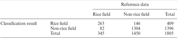
Kappa analysis is one of the most popular methods for determining accuracy, error and agreement between remotely sensed classifications and reference data (Congalton and Green 1999). To apply the kappa analysis, an error matrix for the classification result was created. After the images were classified, we took 1795 points (2% of the total MODIS pixels) from a stratified random sample of rice field and non-rice field classes. The error matrices are shown in table 5.

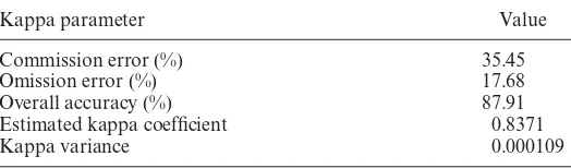
From the error matrices, the commission error, omission error and overall accu-racy were calculated using equations (10)–(12). The algorithm developed in this study had commission error, omission error and overall accuracy of 35.45%, 17.68% and 87.91%, respectively. Furthermore, the estimated kappa coefficient and kappa coeffi-cient variance were calculated using equations (13) and (14) and values of 0.8371 and

(a₎ ₍b₎ Analysis result (ha) Analysis result (ha)

Reference data (ha) Reference data (ha)

0 4 000 8 000 12 000

0 2000 4000 6000 8000 10 000

Figure 6. Relationship between rice area from the reference data and the data produced from this analysis at the regency (a) and district (b) level.

Table 5. Error matrices of the rice field classification results.

Reference data

Rice field Non-rice field Total

Classification result Rice field 263 146 409

Non-rice field 82 1304 1396

Total 345 1450 1805

(16)

Table 6. Kappa parameters of the rice field classification results.

Kappa parameter Value

Commission error (%) 35.45

Omission error (%) 17.68

Overall accuracy (%) 87.91

Estimated kappa coefficient 0.8371

Kappa variance 0.000109

0.000109, respectively, were obtained (table 6). The overall accuracy of more than 80% and the estimated kappa of more than 0.8 demonstrate strong agreement between the remotely sensed classification and the reference data (Congaltonet al. 1983, Lillesand and Kiefer 2000).

4. Conclusions

The temporal variability of the VIs used in this study was higher for irrigated and non-irrigated rice fields compared with other land uses. From the three VIs evaluated, NDVI emerged as the best choice for rice field mapping because of the large difference between the variance of the rice classes and that of the other land-use or land-cover classes. Using variance threshold values from 0.0138 to 0.0208 provided the best rice field classification results. Regression analysis showed that the method in this study produced highR2_{values of 0.9749 and 0.9229 for the regency and district level}

com-parison, respectively. The method in this study also produced low RSME values of 1570.70 and 551.36 ha for the regency and district level comparisons, respectively. The overall accuracy of the method in this study was 87.91%. The commission and omission errors were 35.45% and 17.68%, respectively. Kappa analysis demonstrated strong agreement between the results of the analysis of the MODIS data using the method developed in this study and the reference data, with a kappa coefficient value of 0.8371. This study shows that temporal variance analysis is one of the best-suited methods to map rice areas.

Acknowledgements

This study is funded by the Japan Society for the Promotion of Science (JSPS). We thank the three reviewers for their comments and suggestions on the earlier version of the manuscript.

References

ATKINSON, P.M. and LEWIS, P., 2000, Geostatistical classification for remote sensing: an

introduction.Computers and Geosciences,26, pp. 361–371.

BACHELET, D., 1995, Rice paddy inventory in a few provinces of China using AVHRR data.

Geocarto International,10, pp. 23–38.

BARET, F. and GUYOT, G., 1991, Potentials and limits of vegetation indices for LAI and APAR

assessment.Remote Sensing of Environment,35, pp. 161–173.

BOSCHETTI, M., STROPPIANA, D., BRIVIO, P.A. and BOCCHI, S., 2009, Multi-year monitoring

of rice crop phenology through time series analysis of MODIS images.International Journal of Remote Sensing,30, pp. 4643–4662.

(17)

BOUVET, A., LETOAN, T. and LAM-DAO, N., 2009, Monitoring of the rice cropping system in

the Mekong Delta using ENVISAT/ASAR dual polarization data.IEEE Transactions on Geoscience and Remote Sensing,47, pp. 517–526.

CONGALTON, R.G. and GREEN, K., 1999,Assessing the Accuracy of Remotely Sensed Data:

Principles and Practices, pp. 43–70 (Boca Raton, FL: Lewis Publishers).

CONGALTON, R.G., ODERWALD, R.G. and MEAD, R.A., 1983, Assessing Landsat classification

accuracy using discrete multivariate analysis statistical techniques.Photogrammetric Engineering and Remote Sensing,49, pp. 1671–1678.

FANG, H., 1998, Rice crop area estimation of an administrative division in China using remote

sensing data.International Journal of Remote Sensing,17, pp. 3411–3419.

FANG, H., WU, B., LIU, H. and XUAN, H., 1998, Using NOAA AVHRR and Landsat

TM to estimate rice area year-by-year. International Journal of Remote Sensing,3, pp. 521–525.

FOODCROPSAGRICULTUREDEPARTMENT, 2006,Annual Report of Food Crops, pp. 125–135

(Bali Province: Department Agriculture of Local Government).

GUPTA, R.K., 1993, Comparative study of AVHRR ratio vegetation index and normalized

dif-ference vegetation index in district level agriculture monitoring.International Journal of Remote Sensing,14, pp. 53–73.

HUETE, A., DIDAN, K., MIURA, T., RODRIGUEZ, E.P., GAO, X. and FERREIRA, L.G., 2002,

Overview of the radiometric and biophysical performance of the MODIS vegetation indices.Remote Sensing of Environment,83, pp. 195–213.

HUETE, A.R., 1988, A soil-adjusted vegetation index (SAVI).Remote Sensing of Environment,

25, pp. 295–309.

HUETE, A.R. and ESCADAFAL, R., 1991, Assessment of biophysical soil properties through

spectral decomposition techniques.Remote Sensing of Environment,35, pp. 149–159. HUETE, A.R. and WARRICK, A.W., 1990, Assessment of vegetation and soil water regimes in

partial canopies with optical remotely sensed data.Remote Sensing of Environment,32, pp. 115–167.

HUTCHINSON, C.F., 1982, Techniques for combining Landsat and ancillary data for

digi-tal classification improvement.Photogrammetric Engineering and Remote Sensing,8, pp. 123–130.

JENSEN, J.R., 1986, Introductory Digital Image Processing: A Remote Sensing Perspective,

pp. 205–220 (Upper Saddle River, NJ: Prentice-Hall).

KHUSH, G.S., 2005, What it will take to feed 5 billion rice consumers in 2030.International

Journal of Molecular Biology,59, pp. 1–6.

LETOAN, T., RIBBES, F., WANG, L.F., FLOURY, N., DING, K.H., KONG, J.A., FUJITA, M. and

KUROSU, T., 1997, Rice crop mapping and monitoring using ERS-1 data based on

experiment and modeling results.IEEE Transactions on Geoscience and Remote Sensing, 35, pp. 41–56.

LIEW, S.C., KAM, S.P., TUONG, T.P., CHEN, P., MINH, V.Q., BALABABA, L. and LIM, H., 1998,

Application of multitemporal ERS-2 synthetic aperture radar in delineating rice crop-ping systems in the Mekong River Delta, Vietnam.IEEE Transactions on Geoscience and Remote Sensing,36, pp. 1412–1420.

LILLESAND, T.M. and KIEFER, R.W., 2000, Remote Sensing and Image Interpretation,

pp. 715–735 (New York: John Wiley & Sons).

MAS, J.F. and RAMÍREZ, I., 1996, Comparison of land use classifications obtained by visual interpretation and digital processing.ITC Journal,4, pp. 278–283.

MATTHEWS, R.B., WASSMANN, R., KNOX, J.W. and BUENDIA, L.V., 2000, Using a crop/soil

simulation model and GIS techniques to assess methane emissions from rice fields in Asia: upscaling to national levels.Nutrient Cycling in Agroecosystems, 58, pp. 201–217.

NATIONALLANDAGENCY, 2008,Land Use Map of Bali Province, pp. 1–2 (Bali Province: Local

Government of National Land Agency).

(18)

NIEL, T.G.V. and MCVICAR, T.R., 2001, Remote sensing of rice-based irrigated agriculture: a

review, Rice CRC Technical Report P1105-01/01. Available online at: www.ricecrc.org (accessed 5 October 2009).

NIEL, T.G.V., MCVICAR, T.R., FANG, H. and LIANG, S., 2003, Calculating environmental

mois-ture for per-field discrimination of rice crops.International Journal of Remote Sensing, 24, pp. 885–890.

OKAMOTO, K. and KAWASHIMA, H., 1999, Estimation of rice-planted area in the tropical zone

using a combination of optical and microwave satellite sensor data.International Journal of Remote Sensing,5, pp. 1045–1048.

PAN, X.Z., UCHIDA, S., LIANG, Y., HIRANO, A. and SUN, B., 2010, Discriminating different

landuse types by using multitemporal NDXI in a rice planting area. International Journal of Remote Sensing,31, pp. 585–596.

STRAHLER, A.H., BOSCHETTI, L., FOODY, G.M., FRIEDL, M.A., HANSEN, M.C., HEROLD,

M., MAYAUX, P., MORISETTE, J.T., STEHMAN, S.V. and WOODCOCK, C.E., 2006, Global land cover validation: recommendations for evaluation and accuracy assess-ment of global land cover maps. Available online at: www.nofc.cfs.nrcan.gc.ca/ gofc-gold/Report Series/GOLD_25.pdf (accessed 25 July 2009).

TINGTING, L. and CHUANG, L., 2010, Study on extraction of crop information using time-series

MODIS data in the Chao Phraya Basin of Thailand.Advances in Space Research,45, pp. 775–784.

XIAO, X., BOLES, S., LIU, J., ZHUANG, D., FROLKING, S., LI, C., SALAS, W. and MOORE, B., 2005, Mapping paddy rice agriculture in southern China using multi-temporal MODIS images.Remote Sensing of Environment,95, pp. 480–492.

XIAO, X., BRASWELL, B., ZHANG, Q., BOLES, S., FROLKING, S. and MOORE, B., 2003,

Sensitivity of vegetation indices to atmospheric aerosols: continental-scale observations in Northern Asia.Remote Sensing of Environment,84, pp. 385–392.

XIAO, X., HE, L., SALAS, W., LI, C., MOORE, B. and ZHAO, R., 2002, Quantitative

rela-tionships between field-measured leaf area index and vegetation index derived from VEGETATION images for paddy rice fields.International Journal of Remote Sensing, 23, pp. 3595–3604.

YANG, C.M., LIU, C.C. and WANG, Y.W., 2008, Using Formosat-2 satellite data to estimate

leaf area index of rice crop. Journal of Photogrammetry and Remote Sensing, 13, pp. 253–260.