Tracking Control for Hybrid System of Unmanned
Small Scale Helicopter Using Predictive Control
Sutrisno
1, Salmah
2, Endra Joelianto
3, Agus Budiyono
4, Indah E. Wijayanti
5, Noorma Y. Megawati
6.
1Dept. of Mathematics Education Sanata Dharma University
Yogyakarta, Indonesia [email protected] [email protected]
2,5,6
Dept. of Mathematics Gadjah Mada University Yogyakarta, Indonesia 2
3
Instrumentation & Control Research Group Bandung Institute of
Technology Bandung, Indonesia [email protected]
4
Dept. of Aerospace Information Engineering
Konkuk University Seoul, South Korea [email protected]
Abstract— In this paper, we formulate the hybrid dynamic of unmanned small scale helicopter (Yamaha R-50) as piecewise affine (PWA) model and transform it into equivalent mixed logical dynamic (MLD) model using hybrid system description language (HYSDEL) integrated with hybrid toolbox for MATLAB. This hybrid model is triggered by the location of this unmanned aerial vehicle (UAV) which has two modes. By using the MLD model, we design the controller using model predictive control (MPC) to calculate the optimal control action so that this UAV flights and tracks a trajectory. Finally, we simulate this UAV and its controller to track a rectangular trajectory. From the simulation results, this unmanned small scale helicopter follows given trajectory very well.
Keywords—tracking of hybrid systems; unmanned small scale helicopter; piecewise affine systems; mixed logical dynamic systems, model predictive control.
I. INTRODUCTION
Unmanned small scale helicopter is an unmanned aerial vehicle (UAV) that has been developed for several applications like trajectory tracking, obstacle avoidance, etc. The mathematical model of unmanned small scale helicopter can be represented as a nonlinear model that can be linearized as several linear time invariant state spaces based on the initial speed at trim condition [1,2]. For case when the UAV flies at several conditions (modes), locations in this case, it needs to switch from one dynamic to another generated by UAV’s location. Hence, the dynamic of this UAV can be represented as hybrid model. To control the hybrid model of UAV, we can use a control method for hybrid system.
Hybrid model of this UAV is triggered by the state of the system, so it can be presented in the piecewise-affine (PWA) form. The modes in PWA are depend on the current location of the state vector [3,4]. PWA model can be transformed equivalently into mixed logical dynamic (MLD) form that more suitable for control design and optimization [5,4,6]. This conversion can be done by typing the PWA model in hybrid systems description language (HYSDEL) and obtain its equivalent MLD by using function mld in hybrid toolbox for MATLAB given by [6]. The MLD model contains some auxiliary variables that are binary and real variables and some
inequality constraints. It will affect to the optimization problem that will occur. But, this MLD model is more suitable for control method likes model predictive control (MPC) rather than if we used PWA model [4].
The formulation steps of MPC for MLD is similar to MPC for linear system given by [7] that are predicting the state, input, auxiliary variables and output of MLD model, substituting them into some objective function and minimizing this objective function using an optimization method. The objective function of MPC for MLD is defined as quadratic form that represented the deviation of the state, input, auxiliary variables and output from their reference trajectory [8]. This objective function will be minimized using some optimization method. Since MLD model contains real and integer variables, this optimization problem can be done using mixed integer quadratic programming (miqp) that was embedded in hybrid toolbox for MATLAB given by [6]. The solution of this optimization gives the optimal control value that will be applied to the UAV.
Unmanned small scale helicopter that we will use for simulation is Yamaha R-50. The dynamic of this UAV was appeared in [1,8]. Some applications were applied using this UAV like tracking control [9], obstacle avoidance [10], switched control [1], safety analysis [11], etc. Reference [9] gives tracking control using linear model (non-hybrid) with assumption that the flight area is uniform, so it was done by using one dynamic and it is not needed to switch the dynamic. Trajectory tracking of linear hybrid systems had been developed using some methods and some applications like internal model principle approach [12], tracking via embedding of known reference trajectories [13], by means of internal model principle studied in [14], tracking with unilateral position constraint inducing dissipative impacts [15], etc.
In this paper, we simulate an unmanned small scale helicopter (Yamaha R-50) using hybrid system approach with two modes to track a rectangular reference trajectory. We define these modes as two flight locations that each location has different dynamic. We formulate the PWA model, convert it into MLD using HYSDEL and control this MLD model 2013 International Conference on Robotics, Biomimetics, Intelligent Computational Systems (ROBIONETICS)
Yogyakarta, Indonesia, November 25-27, 2013
using MPC for MLD so that this UAV tracks given reference trajectory. To solve the optimization corresponding to MPC for MLD, we use miqp function embedded in hybrid toolbox for MATLAB.
II. DYNAMICS OF UNMANNED SMALL SCALE HELICOPER We will use the linear model of unmanned small scale helicopter (Yamaha R-50) consist of two models that were appeared in [2] as follow. Let µ be the state vector of the helicopter with
[
u, , , , , , , , , ,]
= w q a v p r b T
µ θ φ ψ (1)
where u and v are the translational fuselage motions, p and q are the angular fuselage motions, w is the rigid body state, r is
yaw rate, ψ defined by d r dt
ψ
= , φ and θ are the angles of
lateral and longitudinal translations respectively, a and b are the rotor state for lateral and longitudinal flapping motions respectively. The helicopter inputs are cyclic collective (δcoll),
cyclic pedal (δped ), cyclic longitudinal (δlong ) and cyclic
lateral (δlat), hence the input vector of this UAV is T
coll long ped lat
u=⎡⎣δ δ δ δ ⎤⎦ (2)
The body coordinate state in XYZ coordinate is
[
x( ), y( ), z( ) t t t]
T =[
u( ), ( ), ( ) .t v t w t]
T (3) Then the full state of this UAV is x=[
x y z µ]
. In this paper, we used two modes to form the PWA model. The first mode is using u0 =4 mps, following [2] , the linear model of this UAV for mode-1 is given by1 1
( ) ( ) ( )
x t =A x t +B u t (4)
where A1 and B1 are real constant matrices with appropriate
dimension appeared in Appendix (3). The second mode is using u0 =8 mps. The linear model of this UAV for mode-2 is given by
2 2
( ) ( ) ( )
x t =A x t +B u t (5)
where A2 and B2 are real constant matrices with appropriate
dimension appeared in Appendix (3). The output is given by
( ) ( )
y t =Cx t (6)
where C is real constant matrix appeared in Appendix (3).
Vector
[
x,y,z]
T in (4)-(5) is the position of helicopter in body coordinate (XYZ coordinate) that can be transformed into local coordinate (NEA coordinate) using matrix T1appeared in Appendix (2). Following [9], this transformation can be written as
[
N E A]
T =TI[
x y z]
T (7)where ( , , )N E A =(North East Altitude, , ) is the position of the helicopter in the local coordinate.
III. HYBRID MODEL OF UNMANNED SMALL SCALE HELICOPTER
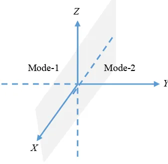
The unmanned small scale helicopter that we used has two modes that are mode-1 associated with (4) and mode-2 associated with (5). We define these modes as follows. We separate the flight area into two different areas that are area-1 ( y≤0) associated with mode-1 and area-2 (y>0) associated with mode-2 that can be illustrated by Figure (1).
Figure 1. Partition of the flight area into two modes
Let k denotes the time instant and x(0)=x0 is the initial state. The dynamic of this UAV can be written as the following PWA model
obtained by discretizing the matrices of systems (4)-(6) using function c2d in MATLAB with time sampling 0.01 s and they are appeared in Appendix (4). For simplicity, we do not change the name of these matrices.
The state and input constraints are given by
30 u 30
By typing (8)-(9) in HYSDEL and converting it into MLD
using mld function given by [6], we have the following
equivalent MLD model
1 2 3
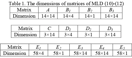
they have the dimensions appeared in Table (1).
Table 1. The dimensions of matrices of MLD (10)-(12)
Matrix A B1 B2 B3
Since the dimension of these matrices are relatively large, we do not append them. This MLD model will be used to control the system using MPC.
IV. MPC FOR MLD
MPC can be applied to control a hybrid system in the MLD form for regulating or trajectory tracking purposes. MPC works by predicting the state, input and output vectors and minimizing some objective function using an optimization method. For tracking problem, the objective function is defined by the state, input and output gains to their reference trajectories. MPC for MLD can be formulated as follows. Assume that MLD model (10)-(12) is controllable and observable. Let Hp be the length of the horizon prediction, then the objective function of MPC for MLD can be defined by
reference trajectories for state, input, auxiliary variables δand
z, and output respectively. The notation v2Q meansv QvT .
The optimization (13) can be transformed into mixed integer quadratic optimization by forming the predictions of state ,x input ,u δ,z and y over horizon prediction Hp and
substituting them into (13). By using some algebraic operation, this transformation gives the following mixed integer quadratic optimization
1 2 0 3 Appendix (1). Optimization (14) can be solved using MIQP solver that was embedded in hybrid toolbox for MATLAB [6]. The optimal solution R* obtained from (14) contains the optimal values for u*, *
δ , and z*. The control action that will be applied to the system is
u
* at current time instant.V. SIMULATION RESULTS
We simulate MLD model (10)-(12) to track a rectangular trajectory. The initial position is
[
0, 0, 0]
[
5,5, 5]
T
N E A = − and
the initial full state is
0 [ ,0 0, , 4,0.001,0, 0.0145,0.0001,0,0,0,0,0,0]0
T
where
[
0, 0, 0]
samples. The weighting matrices for objective function (13) are
, 1, 2, 3, 4, 5
i
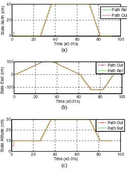
Q =I i= that are identity matrices with appropriate dimension. Simulation results for each state of local coordinate (North, East and Altitude) are given by Figure (2).
Figure 2. Trajectory and the track of the unmanned small scale helicopter, (a) North, (b) East, (c) Altitude
Figure (2) shows the reference trajectories and Helicopter’s track for each local coordinate (N,E,A). From Figure (2), it can be seen that for each axis, helicopter follows the reference trajectory very well. The evolution of the location of the UAV in East coordinate is corresponding to the mode of the hybrid model which means that for time steps approximately 0 to 60, mode-1 was implemented and time steps approximately 60 to 100, mode-2 was implemented.
To view the reference and output trajectories in 3D, we combine North, East and Altitude states into one figure as shown in Figure (3). It can be seen that this helicopter flight from the initial position and then it reaches the reference trajectory in approximately 0.05s and then follows the given reference trajectory in the rectangular shape. Hence, it can be conclude that helicopter tracks the given trajectory well.
Figure 3. Trajectory and track of the unmanned small scale helicopter generated by MPC
VI. CONCLUSIONS AND FUTUR RESEARCH
Tracking control problem of hybrid system of unmanned small scale helicopter (Yamaha R-50) was considered. The hybrid model in the PWA form of this UAV was triggered by the location of the UAV in two modes (two different locations). The MLD model can be converted equivalently from PWA model using HYSDEL. MPC controller was applied to control the MLD model so that this UAV tracks a reference trajectory. The optimization problem corresponding to the MPC for MLD was solved by MIQP. Simulation results show that this helicopter was tracked the given rectangular reference trajectory very well.
In the future researches, we will vary the reference trajectory to be tracked by this UAV to test the robustness and analyze the performance and stability of this controller. Otherwise, we will use more than two modes to formulate the hybrid model of this UAV.
REFERENCES
[1] Sutarto, H.Y., Budiyono, A., Joelianto, E. and Hiong, G.T., 2006, Switched linear control of a model helicopter, Automation, Robotics and Vision proceeding of the international conference in Singapore, December 5-8, 2006, pp. 1300-1307.
[2] E. Joelianto, E. Maryami, A. Budiyono and D. Renaning, 2011, Model Predictive Control for Autonomous Helicopters, Aircraft Engineering and Aerospace Technology (AEAT): An International Journal, Vol 83, Issue 6, pp. 375-387.
[3] Branicky, M. S., Introduction to Hybrid Systems, Department of Electrical Engineering and Computer Science, Case Western Reserve University, Cleveland, OH 44106, U.S.A.
[4] Borrelli, F., Bemporad, A., Morari, M., 2011, Predictive Control for linear and hybrid systems, June 16, 2011.
[7] Maciejowski, J.M., 2002, Predictive Control with Constraints, Prentice Hall Inc., England.
[8] Mettler, B., 2003, Identification Modeling and Characteristic of Miniature Rotorcraft, Kluwer Academic Publishers, Boston, Massachusett, USA.
[9] Budiyono, A. and Wibowo, S.S., 2007, Optimal tracking controller design for a small scale helicopter, Journal of Bionic Engineering, Vol. 4, pp. 271−280.
[10] Salmah, Sutrisno, E. Joelianto, A. Budiyono, I.E., Wijayanti, N.Y. Megawati, Model Predictive Control for Obstacle Avoidance as Hybrid Systems of Small Scale Helicopter, Submitted and Accepted to 2013 3rd
International Conference on Instrumentation, Control and Automation. [11] Salmah, E. Joelianto, N.Y. Megawati, A. Budiyono, H. Y. Sutarto and
Indah E.W., 2010, Safety Analysis of Helicopter Models using Hybrid Systems with Geometric Programming, ICIUS 2010, Nov 3-5, 2010, Bali, Indonesia.
[12] S. Galeani, L. Menini and A. Potini, Trajectory tracking in linear hybrid systems: an internal model principle approach, 2008, American Control Conference Westin Seattle Hotel, Seattle, Washington, USA, June 11-13, 2008.
[13] Ricardo G. Sanfelice, J. J. Benjamin Biemond, Nathan van de Wouw, and W. P. Maurice H. Heemels, 2011, Tracking Control for Hybrid Systems via Embedding of Known Reference Trajectories, American Control Conference on O'Farrell Street, San Francisco, CA, USA, June 29 - July 01, 2011.
[14] Joelianto, E. and D. Williamson, 2009, Transient Response Improvement of Feedback Control Systems using Hybrid Reference Control, International Journal of Control, Vol. 82, No. 10, pp. 1955-1970.
[15] J.J.B. Biemond, N. van de Wouw, W.P.M.H. Heemels, R.G. Sanfelice, and H. Nijmeijer, 2012,Tracking control of mechanical systems with a unilateral position constraint inducing dissipative impacts, 51st IEEE Conference on Decision and Control, December 10-13, 2012. Maui, Hawaii, USA.
[16] Salmah, Solikhatun, Megawati, N.Y., Joelianto, E., Budiyono, A., 2013, Control of Autonomous Helicopter Models with Robust H2-Type
Switched Linear Controller, International Journal of Applied Mathematics and Statistics (IJAMAS), Vol. 35, No. 5, 137-148.
[17] Lazar, M., Heemels, W.P.M.H., Weiland, S. and Bemporad, A., 2006, Stabilizing Model Predictive Control of Hybrid Systems, IEEE Transactions On Automatic Control, Vol. 51, NO. 11, November 2006, pp. 1813-1818.
[18] Bemporad, A., Ferrari-Trecate, G., and Morari, M., 2000, Observability and Controllability of Piecewise Affine and Hybrid Systems, IEEE Transactions On Automatic Control, Vol. 45, NO. 10, October 2000, pp. 1864-1876.
cos cos cos sin sin
sin sin cos cos sin sin sin sin cos cos sin cos
cos sin cos sin sin cos sin sin sin cos cos cos
I
Appendix 3. Matrices of (4)-(6)
1
0 0 0 1 0 0 0 0 0 0 0 0 0 0
0 0 0 0 0 0 0 0 1 0 0 0 0 0
0 0 0 0 1 0 0 0 0 0 0 0 0 0
0 0 0 0.0555 0.0085 0.0010 9.8090 11.4711 0 0 0 0 0 0 0 0 0 0.4699 0.9969 3.9983 0.1419 0.0010 0 0 0 0.6792 0.0769 0 0 0 0 0.1148 0.0231 0.0292 0 223.1810 0 0 0 0 0 0 0 0 0 0.0118 0.0058 0.0009 0.0098 0 0.1362 0.0010 3.9911 9.7854 11.4708 0 0 0 0 0.0198 0.0662 0.0032 0 0 0.1715 0 0.0322 0 420.4654 0 0.11362 35.07 0 0 0.84158 0 4.596 0 8.96576 0 16.657 0 0.02247 0 122.048 0
2
0 0 0 1 0 0 0 0 0 0 0 0 0 0
0 0 0 0 0 0 0 0 1 0 0 0 0 0
0 0 0 0 1 0 0 0 0 0 0 0 0 0
0 0 0 0.167 0.0175 0.0010 9.7738 11.510 0 0 0 0 0 0 0 0 0 0.2500 1.6309 11.9792 0.8403 0.0564 0 0 0 0.5558 0.0633 0 0 0 0 0.4004 0.6571 0.3553 0 223.401 0 0 0 0 0 0
0 0 0 0.0182 0.0091 0.0003 0.0479 0 0.268 0.0010 11.980 9.7580 11.5100 0 0 0 0 0.0550 0.0941 0.0011 0 0 0.2942 0 0.0727 0 420.883 0 0.35564 35.07 0 0 0.76978 0 4.5072 0 8.26462 0 16.336 0 0.26198 0 119.69 0
0 0 0 0
Appendix 4. Matrices of (8)-(9)
1
1 0 0 0.0100 0.0000 0.0000 0.0005 0.0006 0.0000 0.0000 0.0000 0.0000 0.0000 0 0 1 0 0.0000 0.0000 0.0000 0.0000 0.0000 0.0100 0.0000 0.0002 0.0005 0.0006 0 0 0 1 0.0000 0.0100 0.0002 0.0000 0.0001 0.0000 0.0000 0.0000 0.000
A 0 0 0 0.9994 0.0001 0.0001 0.0981 0.1100 0.0000 0.0000 0.0000 0.0000 0.0000 0 0 0 0 0.0047 0.9901 0.0396 0.0016 0.0434 0.0000 0.0000 0.0000 0.0068 0.0007 0 0 0 0 0.0012 0.0002 0.9889 0.0001 2.1328 0.0000 0.0000 0.0000 0.0
− − − −
− − − −
− − 000 0.0000 0
0 0 0 0.0000 0.0000 0.0099 1.0000 0.0108 0.0000 0.0000 0.0007 0.0000 0.0000 0 0 0 0 0.0000 0.0000 0.0096 0.000 0.9094 0.0000 0.0000 0.0000 0.0000 0.0000 0 0 0 0 0.0002 0.0001 0.0000 0.0001 0.0000 0.9984 0.0001 0.03
−
− − − − −
− − −
− − − − − 98 0.0978 0.1099 0
0 0 0 0.0002 0.0007 0.0000 0.0000 0.0000 0.0016 0.9796 0.0004 0.0001 4.0056 0 0 0 0 0.0040 0.0001 0.0002 0.0002 0.0000 0.0125 0.0000 0.9974 0.0006 0.0007 0 0 0 0 0.0000 0.0000 0.0000 0.0000 0.0000 0.0000 0.0099
− − − − −
− −
− − − − −
,
0.0001 1.0000 0.0204 0 0 0 0 0.0000 0.0000 0.0000 0.0000 0.0000 0.0000 0.0095 0.0000 0.0000 0.9001 0 0 0 0 0.1163 0.0000 0.0000 0.0000 0.0000 0.0001 0.0000 0.0100 0.0000 0.0000 1
⎡ ⎤
0.0000 0.0001 0.0000 0.0000 0.0000 0.0000
0.0061 0.0000 0.0000 0.0000 0.0063 0.0196 0.0000 0.0000 1.2225 0.0051 0.0000 0.0017 0.3799 0.0000 0.0000 0.0000 0.0013 0.0004 0.0000 0.0011 0.3352 0.0000 0.0000 0.0084 0.000 0.0886 0.0000 0.1625 0.7147 0.0002 0.0000 1.2187 0.0001 0.0004 0.0000 0.0009 0.0024 0.0004 0.0000 0.0008 0.3341 0.0000 0.0000 0.0061 0.0000
⎡ ⎤
1 0 0 0.0100 0.0000 0.0000 0.0005 0.0006 0.0000 0.0000 0.0000 0.0000 0.0000 0 0 1 0 0.0000 0.0000 0.0000 0.0000 0.0000 0.0100 0.0000 0.0006 0.0005 0.0006 0 0 0 1 0.0000 0.0099 0.0006 0.0000 0.0004 0.0000 0.0000 0.0000 0.0000
A 0 0 0 0.9984 0.0002 0.0001 0.0977 0.1103 0.0000 0.0000 0.0000 0.0000 0.0000 0 0 0 0 0.0022 0.9842 0.1182 0.0084 0.1287 0.0000 0.0000 0.0000 0.0055 0.0006 0 0 0 0 0.0040 0.0065 0.9860 0.0002 2.1325 0.0000 0.0000 0.0000 0.0
− − − −
− − − −
− − − 000 0.0000 0
0 0 0 0.0000 0.0000 0.0099 1.0000 0.0108 0.0000 0.0000 0.0006 0.0000 0.0000 0 0 0 0 0.0000 0.0000 0.0095 0.0000 0.9094 0.0000 0.0000 0.0000 0.0000 0.0000 0 0 0 0 0.0005 0.0001 0.0000 0.0005 0.0000 0.9960 0.0001 0.11
− − − − −
− − − −
− − − − 93 0.0974 0.1101 0
0 0 0 0.0005 0.0009 0.0000 0.0000 0.0001 0.0029 0.9796 0.0009 0.0001 4.0095 0 0 0 0 0.0052 0.0001 0.0001 0.0003 0.0002 0.0215 0.0000 0.9934 0.0010 0.0012 0 0 0 0 0.0000 0.0000 0.0000 0.0000 0.0001 0.0000 0.0099
− − −
− − − −
− − − − −0.0009 1.0000 0.0204 0
0 0 0 0.0000 0.0000 0.0000 0.0000 0.0000 0.0000 0.0095 0.0000 0.0000 0.9001 0 0 0 0 0.0000 0.0000 0.0000 0.0000 0.0000 0.0001 0.0000 0.0100 0.0000 0.0000 1
⎡ ⎤
0.0000 0.0001 0.0000 0.0000 0.0000 0.0000 0.0005 0.0001 0.0070 0.0000 0.0000 0.0000 0.0033 0.0196 0.0000 0.0000 1.3952 0.0152 0.0000 0.0001 0.1914 0.3799 0.0000 0.0000 0.0010 0.0013 0.0003 0.0000 0.0043 0.3352 0.0000 0 B 0.0075 0.0000 0.1165 0.0196 0.0814 0.0000 0.1617 0.7154 0.0028 0.0000 1.1927 0.0001 0.0004 0.0000 0.0013 0.0024 0.0004 0.0000 0.0008 0.3341 0.0000 0.0000 0.0060 0.0000