Prototyping of MODIS LAI and FPAR Algorithm
with LASUR and LANDSAT Data
Yuhong Tian, Yu Zhang, Yuri Knyazikhin, Ranga B. Myneni, Joseph M. Glassy, Gerard Dedieu, and
Steven W. Running
Abstract—This paper describes results from prototyping of the moderate resolution imaging spectroradiometer (MODIS) radiative transfer-based synergistic algorithm for the estimation of global leaf area index (LAI) and fraction of photosynthetically active radiation (FPAR) absorbed by vegetation using land surface reflectances (LASUR) and Landsat data. The algorithm uses multispectral surface reflectances and a land cover classifi-cation map as input data to retrieve global LAI and FPAR fields. Our objectives are to evaluate its performance as a function of spatial resolution and uncertainties in surface reflectances and the land cover map. We analyzed reasons the algorithm can or cannot retrieve a value of LAI/FPAR from the reflectance data and justified the use of more complex algorithms, instead of NDVI-based methods. The algorithm was tested to investigate the effects of vegetation misclassification on LAI/FPAR retrievals. Misclassification between distinct biomes can fatally impact the quality of the retrieval, while the impact of misclassification between spectrally similar biomes is negligible. Comparisons of results from the coarse and fine resolution retrievals show that the algorithm is dependent on the spatial resolution of the data. By evaluating the data density distribution function, we can adjust the algorithm for data resolution and utilize the algorithm with data from other sensors.
Index Terms—Fraction of photosynthetically active radiation (FPAR), land surface reflectances (LASUR), LANDSAT, leaf area index (LAI), moderate resolution imaging spectroradiometer (MODIS).
I. INTRODUCTION
T
HE importance of vegetation in studies of global cli-mate and biogeochemical cycles is well recognized [1]. Presently, most ecosystem productivity models, carbon budget models, and global models of climate, hydrology and bio-geochemistry require vegetation parameters to calculate land surface photosynthesis, evapotranspiration and net primary production [2]–[6]. Therefore, accurate estimates of vegetation parameters are increasingly important in the carbon cycle, the energy balance and environmental impact assessment studies. Two of these parameters are green leaf area index (LAI), a canopy structural variable, and fraction of photosyntheticallyManuscript received June 1, 1999; revised March 1, 2000. This work was sup-ported by the National Aeronautics and Space Administration through MODIS Contract NAS5-96061.
Y. Tian, Y. Zhang, Y. Knyazikhin, and R. B. Myneni are with the Depart-ment of Geography, Boston University, Boston, MA 02215 USA (e-mail: [email protected]).
J. M. Glassy and S. W. Running are with the School of Forestry, University of Montana, Missoula, MT 59812 USA.
G. Dedieu is with CESBIO-Unite mixte CNES-CNRS-UPS, Toulouse, France.
Publisher Item Identifier S 0196-2892(00)06226-4.
active radiation (0.4–0.7 m) absorbed by vegetation (FPAR), a radiometric variable. In order to quantitatively and accurately model global vegetation dynamics and differentiate short-term from long-term trends, as well as to distinguish regional from global phenomena, these two parameters must be collected often for a long period of time and should represent every region of the Earth’s lands [7].
These two parameters are estimated from remote sensing data using empirical relationships between values of LAI/FPAR and vegetation indices which include near-infrared (NIR) to red (RED) band ratios and the normalized difference vegetation index (NDVI) [9]–[15]. The limitations of such methods are well known [16]–[18]. No unique relationship between LAI/FPAR and vegetation index is applicable everywhere and all the time [19]–[21] because the reflectances of plant canopies depend on a number of other factors, such as, measurement geometry and spatial resolution. These empirical relationships are site- and sensor-specific, and are unsuitable for application to large areas or in different seasons [19]. A physically based model to describe the propagation of light in plant canopies and its use in retrieval of biophysical parameters is the preferred al-ternative. In the context of the Earth Observing System (EOS), the land discipline group of the moderate resolution imaging spectroradiometer (MODIS) Science Team is developing algorithms for the determination of landcover, LAI, albedo, etc. to be operationally generated from data from one or more of satellites [22].
One of these algorithms is the synergistic algorithm for the es-timation of global LAI/FPAR from MODIS [7]. At the present time, the algorithm has been developed and theoretically justi-fied, but no evidence of its functionality has been presented. The purpose of this paper is to evaluate the physical functionality and performance of the algorithm by prototyping with the land sur-face reflectances (LASUR) data derived from the advanced very high resolution radiometer (AVHRR) data and Landsat data. Specifically, we would like to know: What is the effect of un-certainties in surface reflectances on the quality of retrieved LAI/FPAR? When and why the algorithm does/does not retrieve a value of LAI/FPAR from the reflectance data? How can an assessment of the algorithm accuracy be made? What is the behavior of the algorithm as a function of spatial resolution? In this paper, first we describe the concepts of the algorithm, the physical meaning of the bidirectional reflectance distribu-tion funcdistribu-tions (BRDF) equadistribu-tion, and the method to adjust the look-up table (LUT). Then the spectral signatures of LASUR and Landsat were analyzed, followed by a series of algorithm prototyping results discussed in the later section.
Results from prototyping are a valuable means of testing the physics of the algorithm and also constitute an important first step toward improving the algorithm. At the most general level, this research contributes to an improved understanding of the algorithm behavior. A more practical benefit is to provide a basis for improved retrieval of surface parameters from satellite data.
II. ALGORITHM
A. Statement of the Problem
The inverse problem of retrieving LAI and FPAR from atmo-spherically corrected BRDF is formulated as follows. Given sun
and view directions, vegetation type, BRDF’s at spectral bands and their uncertainties , find LAI and FPAR. The retrievals are performed by comparing observed and modeled BRDF’s for a suite of canopy structures and soil patterns that cover a range of ex-pected natural conditions. All canopy/soil patterns for which the magnitude of residuals in the comparison does not exceed un-certainties in observed and modeled BRDF’s, i.e.,
(1)
are treated as acceptable solutions to the inverse problem. Here , , are modeled BRDF’s, and [canopy, soil] denotes a canopy/soil pattern, which is unknown and will be discussed later. For each acceptable solution, a value of FPAR is also evaluated. Mean values of LAI and FPAR aver-aged over the set of acceptable solutions are taken as solutions of the inverse problem. A mathematical justification of this pro-cedure is presented in [7]. Its application to the retrieval of LAI and FPAR from multi-angular observation is discussed in [23].
B. Radiation Transport in a Canopy
For MODIS LAI/FPAR algorithm, a three-dimensional (3–D) radiative transfer model is used to derive spectral and angular biome-specific signatures of vegetation canopies. Taking into account features specific to the problem of radiative transfer in plant canopies, powerful techniques developed in nu-clear physics were utilized to split a complicated 3-D radiative transfer problem into two independent, simpler subproblems. The first subproblem describes the radiative regime within the vegetation canopy for the case of a black surface underneath the medium (“black soil problem”). The second subproblem is the radiation field in the vegetation canopy generated by anisotropic heterogeneous wavelength-independent sources located at the canopy bottom (“S problem”). In terms of this approach, the BRDF of a heterogeneous canopy at wavelength can be expressed as [7], [8]
(2)
Here and are directional hemispherical reflectance (DHR) and canopy transmittance for the black soil
problem, and and are reflectance and transmittance resulting from an anisotropic source located underneath the canopy. The weight is the ratio of the BRDF for the black soil problem to , and is the ratio of the canopy leaving radiance generated by anisotropic sources on the canopy bottom to . The weights and are functions of sun-view geometry, wavelength, and LAI. They are precomputed and stored in the LUT [7].
The effective ground reflectance is the fraction of radia-tion reflected by the canopy ground. It depends on the radiative regime at the canopy bottom. However, its range of variations does not exceed the range of variations of the hemispherically integrated bidirectional factor of the ground surface, which is in-dependent of vegetation [7]. Therefore, can be used as a pa-rameter to characterize the ground reflection. The set of various patterns of effective ground reflectances at the MODIS spectral bands is a static table of the algorithm, i.e., the element of the LUT. The present version of the LUT contains 29 patterns of ranging from bright to dark. They were taken from the soil reflectance model developed by Jacquemoud et al.[25], with model inputs presented in Baretet al.[26]. These soil patterns include three soil types: mixtures of clay, sand, and peat. Each soil type is characterized by three moisture levels and three soil roughness types. In biomes with grounds of intermediate bright-ness, all soil patterns are assigned. In biomes where the ground is bright, the first 16 bright soil patterns are used.
Note that and are not included in the LUT. Given canopy absorptance ( and ) and transmit-tance ( and ), they are evaluated via the law of energy conservation as
(3) (4)
This makes canopy reflectance sensitive to the within canopy
radiation regime , , , .
The dependence of canopy absorptance on wavelength for the black soil problem (subscript “bs”) and S problem ( “S”) can be derived [7] as
(5)
Here is the leaf albedo (leaf reflectance leaf transmit-tance). It is a stable characteristic of green leaves, although its magnitude can vary with leaf age and species. In order to ob-tain accurate leaf albedos for the six biome types, we obob-tained leaf spectra data from several sources. Mean leaf reflectance and transmittance values were calculated for the six biome types at seven MODIS bands (645 nm, 859 nm, 469 nm, 555 nm, 1240 nm, 1640 nm, and 2130 nm). We stored the mean albedo in the LUT. Variable is a wavelength independent coefficient de-fined as [7], [27]
Where and are solutions of the black soil problem and S problem for black ( 0) and white ( 1) leaves, and is the extinction coefficient (dependent on vegetation types). is a parallelepiped where vegetation canopies are located. Its height coincides with the height of plants and its horizontal di-mension coincides with the size of the pixels. The coefficient depends on canopy structure and and is an element of the LUT. Because the horizontal dimension of coincides with the size of pixel, is a resolution dependent parameter. A precise derivation of (5), and (6) is given in [7]. Validation of relation-ships (6) with field measurements is presented in [27]. Similar relationships are also valid for canopy transmittance [7], [27].
Thus, given canopy absorptance and transmittance for the black soil problem and S problem at a reference wavelength , one can evaluate these variables at any other wavelength . Therefore, we only store canopy absorptances , transmit-tances , the coefficients , and leaf albedo, instead of and in the LUT. Reflectances and can then be evaluated via the energy conservation law (3) and (4) and in-serted into (2).
Similar to (2), the fraction of radiation absorbed by vegeta-tion, , at wavelength can be expressed as [7]
(7) For each acceptable solution [canopy, soil], a value of FPAR can be explicitly evaluated as the integral of (7) over the photo-synthetically active region of the solar spectrum [7].
C. Physical Meaning of (2)
Any pixel can be depicted as a point in the spectral space. The spectral BRDF’s tend to occupy certain well localized space in the spectral space, depending upon the architecture of the biome. We use (2) to explain this behavior in the RED-NIR plane as follows:
1) If LAI , then ,
, and coincides with bidirectional surface reflectance factor [7]. The BRDF at RED and NIR re-sults from photon-ground interactions. The pixels are located on the so-called soil line (around 1:1 line in the RED-NIR spectral space) [26], [28]. The spectral be-havior for different soil types will determine the exact location of the soil line. The bright soil pattern will gen-erate high reflectance in RED and NIR. The dark soil pattern will generate low reflectance in RED and NIR. 2) A high value of LAI corresponds to a very dense canopy. Its transmittances and are close to zero and thus, the contribution of soil is minimal. Pixels will occupy a narrow space near the NIR axis. Canopy reflectances at RED and NIR wavelengths characterize exactly the spectral properties of vege-tation, that is, plants absorb radiation very efficiently throughout the visible regions and strongly reflect and transmit at NIR. The type of vegetation and its phenology will determine the precise location in the RED-NIR spectral space.
3) If LAI is between case 1) and case 2), neither
nor transmittance will equal zero, and gaps in the vege-tation elements will cause photons to interact with soil and canopies. The soil-canopy interactions will cause the canopy response, with a hypothetical nonreflecting soil background, to shift toward the soil line (RED re-flectance will decrease, and changes in NIR rere-flectance will depend on the soil brightness pattern under the canopy) [28]. The location of pixels will be between the soil line and NIR axis. The more gaps, the smaller the LAI value and the closer the pixels are to the soil line.
To summarize, (2) shows how the location of a pixel in the spectral space is related to LAI values. If a pixel is close to the soil line, its LAI value is small. Away from the soil line toward the NIR axis, the contribution of soil to canopy leaving radiance decreases as the product of and , and thus, LAI values increase. The direction of this movement in the spectral space results in different rates of LAI variations. Such a representation of canopy reflectances is used in our algorithm to build and adjust the LUT, and to interpret results presented in Section IV.
D. Adjusting the LUT for Data Resolution
Before the configurable parameters of the LUT can be set, data of a specific spatial resolution must be analyzed to lo-cate the pixels in the spectral space (for example, the RED-NIR space) according to the biome type. We evaluated the data den-sity distribution function as follows: specifying a fine grid cell in the spectral space, counting the number of canopy reflectances in this cell, and then dividing this value by the total number of pixels in the entire spectral space. The data density distribu-tion funcdistribu-tion was evaluated for each biome type. A locadistribu-tion of high density (25% of all pixels) for each biome in the RED-NIR space was plotted and used to adjust the LUT as follows. The areas of 25% density can be interpreted as the sets of pixels rep-resenting the most probable patterns of canopy structure. As an example, for biome 5 (broadleaf forests), we located the 25% density of this biome in the spectral space during July, the green season. Then we run the algorithm using only these pixels as input data and plotted the histogram of the retrieved LAI value. Based on previously reported results [24], the most probable canopy realization in this case has an LAI value of about 5. It means that the peak of the histogram should be around five. We adjusted the LUT by changing to represent the corresponding data set so that the simulated BRDF at RED and NIR wave-lengths corresponding to LAI fall in the 25% density plot. Given the location of the most probable realization of canopy structure, (2) can be used to specify the location of pixels at other values of LAI and soil patterns. The LUT was then ad-justed for all biomes.
III. DATAANALYSIS
and analyze the surface reflectance data used to prototype the algorithm.
A. Satellite Data
LASUR refers to data acquired during 1989-1990 and pro-cessed at Centre d’Etudes Spatiales de la Biosphere (CESBIO), Toulouse, France, from AVHRR onboard the NOAA-11 satellite [29], [30]. LASUR is a reprocessing of weekly global vegetation index data [31]. AVHRR is a cross-track scanning system fea-turing one visible (RED, 572–698 nm), one NIR (716–985 nm), one short wave infrared, and two thermal infrared channels. For LASUR products, data from RED and NIR channels were used to estimate surface reflectances and vegetation index, and data from the two thermal infrared channels were used to estimate the surface temperature. LASUR data were calibrated and corrected for atmospheric effects and filtered to eliminate residual noises and perturbations [29], [30]. The data span is from 75 N to 55 S in latitude, and 180 W to 180 E in longitude. Each image has 904 rows and 2500 columns. The spatial resolution is 1/7th of a degree. In this study, RED and NIR surface reflectances from July 1989, were used to prototype the MODIS LAI/FPAR al-gorithm. We created a monthly layer based on maximum NDVI compositing of the four weekly layers in this month, minimizing cloud contamination, off-nadir viewing effects, sun-angle ef-fects and aerosol and water vapor efef-fects [32].
A biome classification map (BCM) that describes the global distribution of six canopy structural types (biomes) was used as a prototype of the MODIS land cover product, required by the MODIS LAI/FPAR algorithm. BCM was derived from the AVHRR Pathfinder data set [24] and is time-independent. The six biome types are: grasses and cereal crops (biome 1), shrubs (biome 2), broadleaf crops (biome 3), savannas (biome 4), broadleaf forests (biome 5), and needle forests (biome 6).
We also utilized Landsat Thematic Mapper (TM) scenes of Northwest U S. (Washington and Oregon) from June 26, 1987 at 30 m resolution to evaluate the algorithm’s response to high resolution data. In this study, we used data from band 3 (RED, 630–690 nm) and band 4 (NIR, 760–900 nm). This image was geometrically registered to a terrain-corrected image with an universal transverse Mercator (UTM) projection. The dark object subtraction method of atmospheric correction was used to correct surface reflectance for the atmospheric effect [33], [34]. There was also a “sitemap” containing polygons of known ground cover, associated with this data set. This sitemap distinguished 17 different forest densities, based on the percentage of forest cover in a forested pixel, and seven other types of miscellaneous landcover types. Using the Bayesian maximum likelihood classification method, we separated this image into three biomes, grasses and cereal crops, broadleaf forests and needle forests. We attributed to broadleaf forests all the pixels where hardwood forest makes up more than 60% of the pixel area. Needle forests consist of those pixels in which conifers make up more than 60% of the pixel area. The other landcover classes that do not belong to these three biomes were defined as unknown class types. In total, grasses occupy 6.6% of the total area, and broadleaf and needle forests occupy 4.8% and 10.3% of the total area.
B. Spectral Signatures
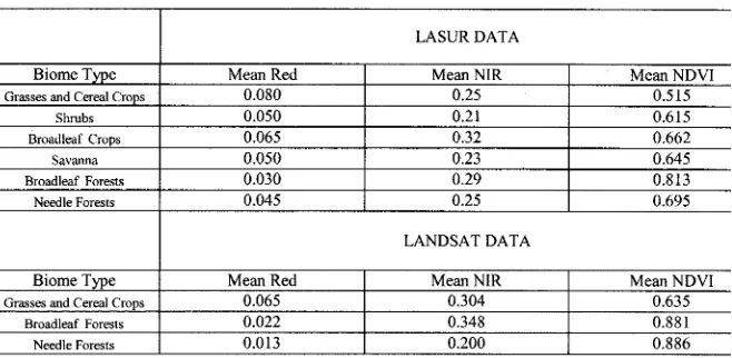
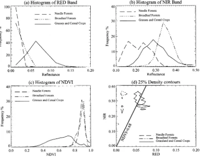
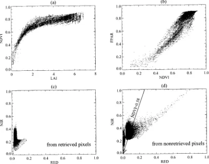
Although all the vegetation types have relatively similar spectral properties (large absorption in RED and large re-flectance in NIR), different biomes have special characteristics depending on the canopy architecture. These characteristics can be distinguished by comparing the spectral signatures. Fig. 1(a) and (b) present histograms of canopy reflectances in RED and NIR spectral bands as a function of biome type derived from LASUR data. In the RED band, canopy reflectances vary between 0.0 and 0.2. Broadleaf and needle forests have the strongest absorption features. On average, they reflect only 3% and 4.5% (Table I) of the incoming radiation. Grasses and broadleaf crops are characterized as the brightest biomes. About 8% and 6.5% of the incoming radiation is reflected. In the NIR band, reflectances vary between 0.1 and 0.5. Shrubs and broadleaf crops represent two extremes. Their reflectances, on average, are 21% and 32%, respectively. The other biomes reflect nearly 25% of the incoming radiation and have similar histograms.
Vegetation indices typically capture the absorption contrast across the 650-850 nm wavelength interval through combina-tions of broadband RED and NIR reflectance. The most widely used index in the processing of satellite data is NDVI, defined
as ( ), where and are spectral
reflectance at NIR and RED wavelengths, respectively. It is a measure of chlorophyll abundance and energy absorption [35]. Fig. 1(c) demonstrates the distribution of NDVI values derived from LASUR data. In general, broadleaf forests have the highest NDVI values, around 0.813, followed by needle forest, around 0.695 (Table I). Broadleaf crops and savannas have similar NDVI distributions, and their NDVI values are larger than those of grasses (0.515) and shrubs (0.615). It would be difficult to distinguish broadleaf crops from savannas using only NDVI.
The data density distribution function, introduced earlier in Section II, can be used to indicate the location of a data peak in the spectral space. Fig. 1(d) shows the location of points with high density for different biomes in the RED-NIR space. Each area bounded by the contour represents an area containing the 25% density of the total pixels from a given biome type. Each biome tends to cluster and occupy a well localized space. Broadleaf forests are located at low RED and high NIR area, while grasses are at the high RED and low NIR area. Broadleaf crops and savannas occupy different locations, although their NDVI distributions are comparable. In general, the more unique a location, the better the ability to distinguish each of the vegetation type. The influence of soil is also clear from this panel. Grasses and shrubs are biomes located near the soil line. Broadleaf forests are dense vegetation and located closest to the NIR axis.
Fig. 1. Statistical properties of canopy reflectances for global LASUR data in July 1989. (a) Histogram of canopy reflectances at the RED band. (b) Histogram of canopy reflectances at the NIR band. (c) Histogram of NDVI. (d) 25% density contours in the RED-NIR space, which shows the location of points with high density for different biomes. The straight line represents the place where NDVI are equal to 0.68. Canopy structure varies considerably with the same NDVI value.
TABLE I
SPECTRALSTATISTICS FORLASUR DATA ANDLANDSATTM DATA
among the three biomes, both at RED and NIR. The NDVI values for the three biomes are 0.635, 0.881, 0.886, respectively (Table I). The 25% density contours are tightly clustered occu-pying a small but unique location in the spectral space. At the same time, the clusters are away from the soil line, and closer to the NIR axis. The biomes are well separated that they do not overlap even on the 75% density contour.
Comparing the results from the previous two data sets, we conclude that, as the spatial resolution increases from LASUR
data to Landsat data, the reflectance decreases in the RED band and increases in the NIR band, and consequently, fewer biomes overlap in the RED-NIR spectral space.
IV. PROTOTYPING OF THEALGORITHM
A. Prototyping with LASUR Data
Fig. 2. Statistical properties of canopy reflectances for Landsat TM data of northwest U.S. in June 1987. (a) Histogram of canopy reflectances at the RED band. (b) Histogram of canopy reflectances at the NIR band. (c) Histogram of NDVI. (d) 25% density contours in the RED-NIR space, which shows the location of points with high density for different biomes. The straight line represents the place where NDVI are equal to 0.68.
The objectives are to analyze these fields and situations when the algorithm fails to retrieve a value of LAI/FPAR, and to as-sess the influence of uncertainties in surface reflectances on the LAI/FPAR product quality.
The algorithm was run pixel-by-pixel using LASUR data and land cover BCM on all pixels with NDVI greater than 0.1. The following notions are used in discussion on algorithm perfor-mance. First, a pixel for which the algorithm retrieves a value of LAI is a “retrieved” pixel. Second, a pixel for which the al-gorithm can not retrieve a value of LAI is termed a “nonre-trieved” pixel, and the algorithm is said to have failed for this pixel. Third, the ratio of the number of retrieved pixels to the total number of pixels is the retrieval index (RI).
1) Input Data: Atmospherically-corrected surface re-flectances and uncertainties in measurements and simulations are inputs to the algorithm (1). However, LASUR reports no information on reflectance uncertainties. Therefore, the uncertainties were simulated as
(8)
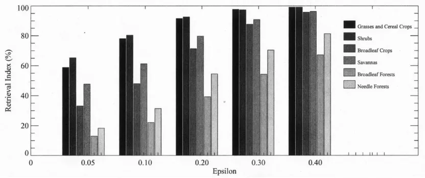
Here, is the mean uncertainty and is assumed to be a constant in this study. Fig. 3 demonstrates the dependence of the RI on . The RI increases with increases in . However, the quality of retrieved LAI/FPAR decreases with increases in . If is under-estimated, the algorithm fails even though surface reflectances
were reasonable. If is overestimated, the algorithm can pro-duce LAI/FPAR values for nonvegetated pixels. Finding for which about 95% of nonretrieved pixels are nonvegetated is a solution to the above problem, which was 0.2 for the LASUR data. The RI varies with biome types at a constant . When is 0.2, the RI for the six biomes is 91.5%, 92.7%, 74.0%, 79.7%, 39.3%, 54.5%, respectively. The reason that broadleaf and needle forests have low RI could be due to dark soil pat-terns used to represent effective ground reflectance in (2). If a pixel is bright, it will not be considered as a pure broadleaf or needle forest pixel and, consequently, the algorithm will fail. Low values of RI are not necessarily an indication of poor per-formance of the algorithm. For the coarse resolution data, such as LASUR (1/7th of a degree), the vegetation in the pixel may be a case of mixture of different land cover classes. Therefore, biome-specific spectral features may be lost. At the present time, restricting the algorithm to pure vegetation types retains the ability to discriminate biome types.
Fig. 3. Dependence of the retrieval index (RI) on uncertainties"in measurements and simulations.
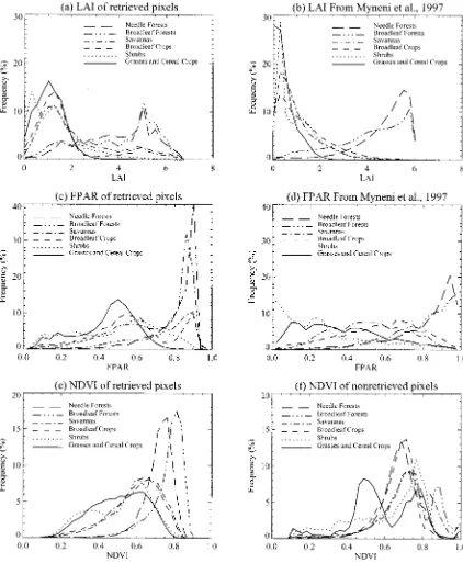
are seen in the peak and tail of the LAI histograms. The highest frequency of LAI for broadleaf crops and savannas is around 1.25, for grasses around 1.0, and for shrubs around 0.75 and 1.25. The distribution tail of broadleaf crops and savannas con-tains at least 20% of the pixels whose LAI values are larger than 4.0. The tail ends at about 4.0 for grasses and shrubs. Therefore, the mean LAI for broadleaf crops and savannas are 2.1 and 2.2, for grasses and shrubs, only 1.2 and 1.4. Shrubs have two ob-vious peaks that correspond to the two peaks in the NDVI his-togram shown in Fig. 1(c). However, the retrieved LAI is not based on the NDVI.
The LAI distribution from a NDVI-based algorithm de-veloped earlier by Myneni et al. [24] is shown in Fig. 4(b). The data used for this NDVI-based algorithm were AVHRR Pathfinder data from July 1981 through June 1991. The average July retrievals over the ten-year period are shown in this figure. There are many similarities between Fig. 4(a) and (b). Broadleaf and needle forests have much higher LAI than the other four biomes. The double peak in shrubs is also seen in Fig. 4(b). The similarity between the two retrievals imbues confidence in the MODIS algorithm.
Fig. 4(e) and (f) show the NDVI histograms from retrieved and nonretrieved pixels. Compared to Fig. 1(c), the NDVI his-togram of retrieved pixels is similar to the NDVI hishis-togram of all pixels. Therefore, the algorithm identifies most of the features in the observed data. Failures are typically two cases. First, NDVI is too high for a particular biome. For example, the algorithm fails to retrieve information when the NDVI of grasses is larger than 0.75. In the LUT, there is no information for grasses at such values of NDVI. Second, for the same NDVI value, some of the pixels are retrieved pixels, but the others are not. The failure of this type will be discussed later.
3) Test of Physics: There are many examples in published literature about the strong relation between NDVI and LAI and FPAR [9]–[15]. This provides an opportunity to test the physics of the algorithm by comparing the LAI-NDVI and FPAR-NDVI relationships derived from the algorithm with those reported from field measurements. Fig. 5(a) and (b) shows the distributions of the retrieved values of LAI and FPAR with respect to the NDVI of biome 5. LAI is nonlinearly proportional
to NDVI, while FPAR is linearly proportional to NDVI. This corresponds to relations reported in the literature [24], [36]. Note the NDVI in this plot is evaluated from measured RED and NIR reflectances, while the retrieved quantities result from the algorithm that uses reflectances instead of NDVI. The advantages of using the MODIS algorithm instead of NDVI relations are as follows. First, NDVI–LAI relations are subject to changes in sun angle, background reflectance, and view angle, while the MODIS algorithm actually uses these changes as sources of information in the retrieval process. Second, NDVI is based on two spectral bands only, while the algorithm can ingest 3, 4, or even MODIS 7 bands simultaneously to retrieve LAI and FPAR.
Fig. 4. (a), (c) Histograms of LAI/FPAR derived from the MODIS algorithm with LASUR data. (b), (d) Histograms of LAI/FPAR derived from NDVI-based algorithm with ten-year averaged AVHRR Pathfinder data [24]. (e) Histogram of NDVI from retrieved pixels. (f) Histogram of NDVI from nonretrieved pixels. The mean uncertainty"is 0.20.
4) Reliability of Retrieved LAI/FPAR: Equation (1) may admit a number of solutions, covering a wide range of LAI values. When this happens, the canopy reflectances are said to belong to the saturation domain, being insensitive to various parameter values characterizing the canopy. The algorithm can recognize this situation. The frequency with which LAI values are retrieved under the condition of saturation is termed satura-tion frequency. The accuracy of retrievals decreases in the case of saturation, that is, the information conveyed about canopy structure by canopy reflectances is small because a wide range
Fig. 5. For broadleaf forests in LASUR data, the scatter plot shows (a) the LAI-NDVI relationship, (b) the NDVI-FPAR relationship, (c) retrieved pixels in the RED-NIR space, and (d) nonretrieved pixels in the RED-NIR space.
Fig. 6. (a) Histogram of LAI values retrieved under the condition of saturation. Solid lines present the same histograms as Fig. 4(a). Dashed lines show the ratio of the number of LAI values retrieved under the condition of saturation to the total number of retrieved pixels. (b) Coefficient of variation (standard deviation/mean) of retrieved LAI values (COVLAI) as a function of retrieved LAI.
Nearly every pixel is retrieved under the condition of saturation when the LAI is larger than 5.0.
Broadleaf and needle forests in general have high LAI values, and therefore, a high saturation frequency. In order to assess the quality of retrieved LAI/FPAR values, we examine the coeffi-cient of variation of the retrieved LAI value (COVLAI) defined
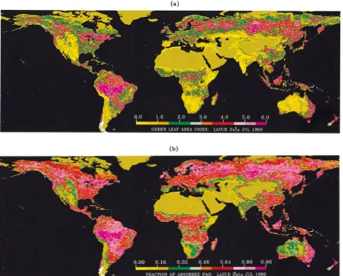
be-Fig. 7. (a) Global LAI and (b) global FPAR fields derived from LASUR data in July, 1989. For the nonretrieved pixels, the LAI-NDVI, and NDVI-FPAR relations were used to estimate LAI and FPAR.
cause at high LAI values the reflectances belong to the satura-tion domain and it is difficult to localize a single estimate. When LAI is larger than 3.0, broadleaf and needle forests have rela-tively lower COVLAI values than other biomes at the same LAI value. Therefore, when LAI is large and saturation frequency is large, the retrieval is not necessarily poor. COVLAI cannot be less than 0.2, because the mean uncertainty in these runs is 0.2. The quality of the retrievals cannot be better than the quality of the largest uncertainty in spectral reflectance data input to the algorithm. Therefore, the availability of band specific uncertain-ties in atmospherically corrected surface reflectances is critical to assess the quality of the LAI/FPAR product.
5) LAI and FPAR Images: The algorithm was run on the global LASUR data for the month of July 1989. For the nonre-trieved pixels, the averaged NDVI-LAI/NDVI-FPAR relations derived from all the retrieved pixels were used to estimate LAI and FPAR. Fig. 7 shows color-coded images of global LAI and FPAR. These compare well with the fields reported earlier by Myneni et al.[24]. The comparison was done to assess if the algorithm captures the general patterns of LAI and FPAR
dis-tribution at the global scale. Whether the retrievals are accurate or not requires validation, which is the next step.
misclas-TABLE II
(a) SUCCESSINDEX AND(b) MEANLAIFORMISCLASSIFIEDLASUR DATA
sification happens between spectrally and structurally similar biomes, perhaps, because of coarse spatial resolution, the impact on LAI/FPAR retrievals is difficult to assess. As an example, consider shrubs (biome 2) and savannas (biome 4). The RI and mean LAI do not vary greatly. The retrieved LAI/FPAR values are acceptable, although the pixels have been misclassified. This example indicates that various biome LUT’s share similar en-tries for certain combinations of spectral reflectances.
B. Prototyping with Landsat Data
1) General Results: The MODIS LAI/FPAR algorithm was prototyped with Landsat data for three biomes: grasses and ce-real crops, broadleaf forests, needle forests. A fine resolution LUT was used to retrieve LAI and FPAR because of the finer spatial resolution of Landsat data. The RI’s for the three veg-etation types are 90.7%, 53.9%, 57.9%, respectively, and the mean LAI values are 1.87, 5.79, 4.11, respectively. Compared to
LASUR data, the RI increase for broadleaf and needle forests, and so do the mean LAI values. The saturation frequencies at high LAI values for these biomes are comparable to those re-ported earlier for LASUR data.
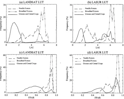
Fig. 8. Retrievals from Landsat data as a function of spatial resolution-dependent look-up table (LUT). Histograms of LAI from (a) Landsat LUT, (b) LASUR LUT, (c) histograms of FPAR from Landsat LUT, and (d) LASUR LUT.
LUT on the spatial resolution of data. To further investigate, the algorithm was performed on Landsat data with LASUR LUT, that is, fine resolution data with coarse resolution LUT. Fig. 8 shows the histogram of LAI and FPAR obtained from Landsat data with LASUR LUT and, also, Landsat data with Landsat LUT. When Landsat data and Landsat LUT are used, the re-trieved LAI values vary from 0.0 to 2.5 for grasses, from 5.0 to 7.0 for broadleaf forest, and from 1.5 to 6.0 for needle forests (Table III). When LASUR LUT is used with Landsat data, the histograms of retrieved LAI and FPAR change greatly. For ex-ample, the LAI of grasses/cereal crops can reach unrealistic values between 4.0 and 6.0. The LAI of needle forests is con-centrated between 1.5 to 4.0, a relatively small range for this biome. The RI for the three biomes also decrease to 87.5%, 39.2%, 4.7%, respectively. When the algorithm is run using LASUR data but with Landsat LUT (Fig. 9), the mean LAI for all biomes decrease, and the differences between forests (high LAI) and other biomes (low LAI) disappear. FPAR shows sim-ilar changes. This clearly indicates the dependency between data resolution and the LUT.
2) Soil or Background Effects: As previously mentioned, in the design of the MODIS LAI/FPAR algorithm, the 3-D ra-diative transfer problem can be represented as the sum of two components. The first describes the radiation regime within the vegetation canopy with a completely absorbing soil or back-ground beneath the canopy. The second component describes
additional radiation due to interactions between the soil and vegetation. Therefore, the soil-vegetation interaction is an im-portant component controlling the spectral behavior of vege-tation canopies. At the fine resolution, the contribution of the soil-vegetation interaction is negligible in the case of dense veg-etation, such as forests. We executed the algorithm only with the black soil problem on Landsat data to test this assumption. The RI can be as high as 50.6% (broadleaf forest) and 54.3% (needle forest), compared to 53.7% and 57.9% if the contri-bution from the soil-vegetation interaction is added. The his-tograms of retrieved LAI and FPAR do not change substan-tially. Therefore, the fine resolution Landsat data represent pure and dense vegetation with minimal soil or background effects in this instance. The RI are only 31% and 45% for broadleaf and needle forests when only the black soil problem is used to retrieve LAI and FPAR for the coarser resolution LASUR data. The soil-vegetation interaction is an important component that controls the spectral behavior of vegetation canopies. Its effect becomes large as the resolution decreases.
V. CONCLUSIONS
TABLE III
COMPARISON OFTHERESULTSFROMLASUR LUTANDLANDSAT LUT RETRIEVALS
Fig. 9. Retrievals from LASUR data using Landsat look-up table (LUT). Histograms of (a) LAI and (b) FPAR.
savannas 2.1 and 2.2, shrubs 1.4 and grasses and cereal crops 1.2. The algorithm utilizes leaf spectral properties and canopy structural attributes, instead of NDVI, in the retrieval process. An LAI value can only be retrieved when a pixel falls within the specified spectral and angular space in the LUT.The algorithm fails even if the NDVI value is reasonable. The uncertainties in input data influence the RI. RI increases with increasing uncer-tainties. However, the quality of retrieved LAI/FPAR decreases with increasing uncertainties. A value of 0.2 was found optimal in this study. Quantitatively, the saturation frequency and coef-ficient of variation (standard deviation/mean) of retrieved LAI values (COVLAI) are two useful metrics to assess the quality of the retrieved field. The higher the saturation frequency and COVLAI value, the lower the quality of the retrieval. On av-erage, if LAI is larger than 4.0, saturation problems begin to in-fluence the retrieval. Forests have higher saturation frequencies than other vegetation types. However, they have lower COVLAI values than other biomes at the same LAI value, especially at high LAI values. Therefore, the retrieval quality is not neces-sarily poor. COVLAI cannot be less than the total uncertainty in
the data and the LUT, because the quality of the retrievals cannot be better than the quality of the largest uncertainty in spectral re-flectance data input to the algorithm. The effect of biome mis-classification between distinct biomes on the algorithm can be evaluated through the RI, mean LAI, and the histogram of the re-trieved LAI distribution. Misclassification can fatally impact the quality of the retrieval in this case. The impact of biome misclas-sification between spectrally and structurally similar biomes is negligible, particularly if the spatial resolution of the input data is coarse.
ACKNOWLEDGMENT
The authors would like to thank Dr. M. Pax-Lenney and Dr. C. E. Woodcock for the Landsat TM data, as well as two anony-mous reviewers for their careful critiques, which greatly im-proved the quality and readability of the manuscript.
REFERENCES
[1] P. J. Sellers and D. S. Schmid, “Remote sensing of the land biosphere and biogeochemistry in the EOS era: Science priorities, methods and im-plementation—EOS land biosphere and biogeochemical cycles panels,”
Global Planetary Change, vol. 7, pp. 279–297, 1993.
[2] C. S. Potter, J. T. Randerson, C. B. Field, P. A. Matson, P. M. Vitousek, H. A. Mooney, and S. A. Klooster, “Terrestrial ecosystem production: A process model based on global satellite and surface data,”Global
Bio-geochem. Cycles, vol. 7, pp. 811–841, 1993.
[3] S. D. Prince, “A model of regional primary production for use with course resolution satellite data,” Int. J. Remote Sens., vol. 12, pp. 1313–1330, 1991.
[4] P. J. Sellers, R. E. Dickinson, D. A. Randall, A. K. Betts, F. G. Hall, J. A. Berry, G. J. Collatz, A. S. Denning, H. A. Mooney, C. A. Nobre, N. Sato, C. B. Field, and A. Henderson-Sellers, “Modeling the exchange of energy, water, and carbon between continents and atmosphere,”Science, vol. 275, pp. 602–609, 1997.
[5] S. W. Running and J. C. Coughlan, “A general model of forest ecosystem processes for regional applications. I. Hydrologic balance, canopy gas exchange and primary production processes,”Ecol. Model, vol. 42, pp. 125–154, 1988.
[6] S. W. Running and S. T. Gower, “FOREST-BGC, a general model of forest ecosystem processes for regional applications, II. Dynamic carbon allocation and nitrogen budgets,”Tree Phys., vol. 9, pp. 147–160, 1991. [7] Y. Knyazikhin, J. V. Martonchik, R. B. Myneni, D. J. Diner, and S. Run-ning, “Synergistic algorithm for estimating vegetation canopy leaf area index and fraction of absorbed photosynthetically active radiation from MODIS and MISR data,”J. Geophys. Res., vol. 103, pp. 32 257–32 275, 1998.
[8] Y. Knyazikhin, J. V. Martonchik, D. J. Diner, R. B. Myneni, M. M. Ver-straete, B. Pinty, and N. Gobron, “Estimation of vegetation canopy leaf area index and fraction of absorbed photosynthetically active radiation from atmosphere-corrected MISR data,”J. Geophys. Res., vol. 103, pp. 32 239–32 256, 1998.
[9] G. Asrar, M. Fuchs, E. T. Kanemasu, and J. L. Harfield, “Estimating absorbed photosynthetic radiation and leaf area index from spectral re-flectance in wheat,”Agron J., vol. 76, pp. 300–306, 1984.
[10] C. J. Tucker and P. J. Sellers, “Satellite remote sensing of primary pro-duction,”Int. J. Remote Sens., vol. 7, pp. 1395–1416, 1986.
[11] D. L. Peterson, M. A. Spanner, S. W. Running, and L. Band, “Relation-ship of Thematic Mapper Simulator data to leaf area index,”Remote
Sens. Environ., vol. 22, pp. 323–341, 1987.
[12] S. B. Verma, P. J. Sellers, C. L. Walthall, F. G. Hall, J. Kim, and S. J. Goetz, “Photosynthesis and stomatal conductance related to reflectance on the canopy scale,”Remote Sens. Environ., vol. 44, pp. 103–116, 1993. [13] R. B. Myneni and D. L. Williams, “On the relationship between FAPAR
and NDVI,”Remote Sens. Environ., vol. 49, pp. 200–211, 1994. [14] J. M. Chen, “Canopy architecture and remote sensing of the fraction of
photosynthetically active radiation absorbed by boral conifer forests,”
IEEE Trans. Geosci. Remote Sensing, vol. 34, pp. 1353–1368, Nov.
1996.
[15] J. M. Chen and J. Cihlar, “Retrieving leaf area index of boreal conifer forests using landsat TM images,”Remote Sens. Environ., vol. 55, pp. 153–162, 1996.
[16] J. C. Price, “Estimating leaf area index from satellite data,”Remote Sens.
Environ., vol. 31, pp. 727–734, 1993.
[17] G. Asrar, R. B. Myneni, and B. J. Choudhury, “Spatial heterogeneity in vegetation canopies and remote sensing of Absorbed Photosynthetically Active Radiation: A modeling study,”Remote Sens. Environ., vol. 41, pp. 85–101, 1992.
[18] G. G. Gutman, “Vegetation indices from AVHRR: An update and future prospects,”Remote Sens. Environ., vol. 35, pp. 121–136, 1991. [19] N. Gobron, B. Pinty, and M. M. Verstraete, “Theoretical limits to the
es-timation of the Leaf Area Index on the basis of visible and near-infrared remote sensing data,”IEEE Trans. Geosci. Remote Sensing, vol. 35, pp. 1438–1445, Nov. 1997.
[20] M. A. Friedl, F. W. Davis, J. Michaelson, and M. A. Moritz, “Scaling and uncertainty in the relationship between NDVI and land surface bio-physical variables: An analysis using a scene simulation model and data from FIFE,”Remote Sens. Environ., vol. 54, pp. 233–246, 1995. [21] M. A. Friedl, “Examining the effects of sensor resolution and sub-pixel
heterogeneity on spectral vegetation indices: Implications for biophys-ical modeling,” inScaling of Remote Sensing Data for GIS, D. A. Quattrochi and M. F. Goodchild, Eds. New York: Lewis, 1996, pp. 113–139.
[22] C. O. Justice, E. Vermote, J. R. G. Townshend, R. Defries, D. P. Roy, D. K. Hall, V. V. Salomonson, J. L. Privette, G. Riggs, A. Strahler, W. Lucht, R. B. Myneni, Y. Knyazikhin, S. W. Running, R. R. Nemani, Z. Wan, A. R. Huete, W. van Leeuwen, R. E. Wolfe, L. Giglio, J.-P. Muller, P. Lewis, and M. J. Barnsley, “The Moderate Resolution Imaging Spectroradiometer (MODIS): Land remote sensing for global change research,”IEEE Trans. Geosci. Remote Sensing, vol. 36, pp. 1228–1240, Jul. 1998.
[23] Y. Zhang, Y. Tian, Y. Knyazikhin, J. V. Martonchik, D. J. Diner, M. Leroy, and R. B. Myneni, “Prototyping of MISR LAI and FPAR and algorithm with POLDER data over Africa,”IEEE Trans. Geosci. Remote
Sensing, vol. 38, pp. 2402–2418, Sept. 2000.
[24] R. B. Myneni, R. R. Nemani, and S. W. Running, “Estimation of Global Leaf Area Index and Absorbed Par Using Radiative transfer Models,”
IEEE Trans. Geosci. Remote Sensing, vol. 35, pp. 1380–1393, Nov.
1997.
[25] S. Jacquemond, F. Barret, and J. F. Hanocq, “Modeling spectral and bidi-rectional soil reflectance,”Remote Sens. Environ., vol. 41, pp. 123–132, 1992.
[26] F. Baret, S. Jacquemond, and J. F. Hanocq, “The soil line concept in remote sensing,”Remote Sens. Rev., vol. 7, pp. 65–82, 1993. [27] O. Panferov, Y. Knyazikhin, R. B. Myneni, J. Szarzhinski, S. Engwald,
K. G. Schnitzler, and G. Gravenhorst, “The role of canopy structure in the spectral variation of transmission and absorption of solar radiation in vegetation canopies,”IEEE Trans. Geosci. Remote Sensing, to be pub-lished.
[28] A. R. Huete, “A Soil-Adjusted Vegetation Index (SAVI),”Remote Sens.
Environ., vol. 25, pp. 295–309, 1988.
[29] B. Berthelot, G. Dedieu, F. Cabot, and S. Adam, “Estimation of surface reflectances and vegetation index using NOAA/AVHRR: Methods and results at global scale,” inProc. Commun. 6th Int. Symp. Physical
Mea-surements and Signatures in Remote Sensing, Val d’Isère, France, Jan.
17–21, 1994.
[30] B. Berthelot, S. Adam, L. Kergoat, F. Cabot, G. Dedieu, and P. Maisongrande, “A global dataset of surface reflectances and vegetation indices derived from AVHRR/GVI time series for 1989–1990: The LAnd SUrface Reflectances (LASUR) data,” inProc. Commun. 7th
Int. Symp. Physical Measurements and Signatures in Remote Sensing.
Courchevel, France, Apr. 7–11, 1997.
[31] G. Gutman, D. Tarpley, A. Ignatov, and S. Olson, “The enhanced NOAA global land dataset from the Advanced Very High-Resolution Radiometer,”Bull. Amer. Meteorol. Soc., vol. 76, pp. 1141–1156, 1995. [32] B. N. Holben, “Charactistics of maximum-value composite images from temporal AVHRR data,”Int. J. Remote Sens., vol. 7, pp. 1417–1434, 1986.
[33] P. S. Chavez, Jr., “Radiometric calibration of Landsat Thematic Mapper multispectral images,”Photogramm. Eng. Remote Sensing, vol. 55, pp. 1285–1294, 1989.
[34] , “Image-based atmospheric corrections—Revisited and im-proved,”Photogramm. Eng. Remote Sensing, vol. 62, pp. 1025–1036, 1996.
[35] R. B. Myneni, F. G. Hall, P. J. Sellers, and A. L. Marshak, “The inter-pretation of spectral vegetation indices,”IEEE Trans. Geosci. Remote
Sensing, vol. 33, pp. 481–486, Mar. 1995.
[36] J. G. P. W. Clevers, “The application of a weighted infrared-red vegeta-tion index for estimating leaf area index by correcting for soil moisture,”
Remote Sens. Environ., vol. 29, pp. 25–37, 1989.
Yuhong Tianreceived the B.S. degree in meteorology from Nanjing Institute of Meteorology, Nanjing, China, in 1992 and the M.S. degree in meteorology from the Chinese Academy of Meteorological Sciences, Beijing, China, in 1995. She is currently pursuing the Ph.D in the Department of Geography, Boston University, Boston, MA, working on prototyping and validating the synergistic algorithm of LAI and FPAR estimation of the MODIS projects.
Yu Zhangreceived the B.S. degree in physics from the Tsinghua University, Beijing, in 1994 and the M.S. degree in electronics from Peking University, Beijing, China, in 1997. He is currently pursuing the Ph.D. degree in the area of remote sensing and vegetation land surface study in the Department of Ge-ography, Boston University, Boston, MA, working on developing, prototyping, and validating the synergistic algorithm of LAI and FPAR estimation for the MODIS and MISR projects.
His research interests are multi-angle remote sensing and radiative transfer models in vegetation canopies.
Yuri Knyazikhinreceived the M.S. degree in applied mathematics from Tartu University, Tartu, Estonia, in 1978, and the Ph.D. degree in numerical analysis from the N.I. Muskhelishvilli Institute of Computing Mathematics, the Georgian Academy of Sciences, Tbilisi, Georgia, in 1985.
From 1978 to 1990, he was a Research Scientist with the Institute of As-trophysics and Atmospheric Physics and the Computer Center of the Siberian Branch of the Russian Academy of Sciences, Tartu University. He was with the University of Göttingen, Göttingen, Germany, from 1990 to 1996. He is cur-rently a Research Associate Professor, Department of Geography, Boston Uni-versity, Boston, MA. He has worked and published in areas of numerical integral and differential equations, theory of radiation transfer in atmospheres and plant canopies, remote sensing of the atmosphere and plant canopies, ground-based radiation measurements, forest ecosystem dynamics, and modeling sustainable multifunctional forest management.
Dr. Knyazikhin was an Alexander von Humboldt Fellow from 1992 to 1993.
Ranga B. Mynenireceived the Ph.D. degree in biology from the University of Antwerp, Antwerp, Belgium, in 1985.
Since 1985, he has been with Kansas State University, Manhattan, the Uni-versity of Göttingen, Göttingen, Germany, and NASA Goddard Space Flight Center, Greenbelt, MD. He is currently on the Faculty of the Department of Ge-ography, Boston University, Boston, MA. His research interests are in radiative transfer, remote sensing of vegetation, and climate-vegetation dynamics.
Dr. Myneni is a MODIS and MISR science team member.
Joseph M. Glassyreceived the M.S. degree in forestry from the University of Montana, Missoula, in 1994.
Before pursuing his degree, he was a Programmer/Systems Analyst with Systems for Environmental Management for ten years, designing and implementing biological and Earth science application software with an emphasis on remote sensing, statistical, and spatial analysis. He is currently the Director of Software Development for the Numerical Terradynamics Simulation Group (NTSG), School of Forestry, University of Montana. At the NTSG, he has been the Lead Software Engineer since 1994, developing the NASA Terra platform MODIS land algorithms for FPAR, LAI, PSN, and NPP. His research interests include high performance computer facility design and implementation, scalable systems engineering and software architecture, and developing ecosystem science software at multiple temporal and spatial scales.
Mr. Glassy is a MODIS Team SCF associate.
Gerard Dedieuwas born in Carcassonne, France, on May 3, 1956. He received the Ph.D degree in astronomy, astrophysics, and space techniques from the Paul Sabatier University (UPS), Toulouse, France, in 1984.
In 1988, he joined the Centre National d’Etudes Spatiales (CNES), Toulouse, working as a Research Scientist with Laratoire d’Etudes et de Recherches en Teledetection Spatiale (LERTS), now the Centre d’Etudes Spatiales de la Biosphére (CESBIO), a joint laboratory of CNES-CNRS and UPS. He specialized first in the preprocessing of satellite measurements (atmospheric effect corrections), developing methods to estimate surface parameters (albedo, solar radiation, net primary productivity) and defining data archives for global change studies. From 1993 to 1999, he was in charge of the coordination of the “Terrestrial Biosphere” component of the European Study of Carbon in the Ocean, Biosphere, and Atmosphere (ESCOBA) Project, funded by the European Commission. His main research interests are currently in the development of assimilation techniques of remotely sensed data within regional and global vegetation functioning and SVAT’s models. He is also working on the improvement of SPOT 4 vegetation preprocessing techniques and products.
Steven W. Runningreceived the B.S. and M.S. degrees from Oregon State Uni-versity, Corvallis, and the Ph.D. degree from Colorado State UniUni-versity, Fort Collins.