236
11
Market Equilibrium
C O N C E P T S
● Excess Demand ● Excess Supply
● Market Equilibrium ● Market Clearing
● Equilibrium Price ● Walrasian Stability
● Marshallian Stability ● Non-sustainable Industry
● Increase in Competition ● Consumer Price
● Producer Price ● Exchange Rate
● Currency Appreciation ● Currency Depreciation
● FAD theory of Famine ● Sen’s Distribution Theory of Famine
● Price Mechanism ● Invisible Hand
● Indirect Intervention ● Direct Intervention
● Control Price ● Rationing
● Shortage ● Support Price or Minimum Support Price
● Public Distribution System ● Targeted Public Distribution System
W
e have studied consumer behaviour and producer behaviour separately. In a market, consumers and producers interact and, therefore, in some sense, their behaviour must be consistent with each other.More specifically, consider the market for, say, chewing gum. From its demand curve we know how much of it will be demanded at various prices. From its sup-ply curve we can tell how much of it will be supplied at different prices. But what will be the actual price of chewing gum prevailing in the market?
In the very long run, when firms can enter into or leave an industry depend-ing on whether profits are made or losses incurred, price equals the minimum long-run average cost (as we saw in Chapter 10). But if we consider a time hori-zon not so long, the price must be influenced by the forces of both demand and supply. That price will prevail in the market at which the quantity demanded of chewing gum is equal to the quantity supplied of it. This is a notion of match-ing the behaviour of producers of chewmatch-ing gum with that of the consumers. It is called market equilibrium (to be defined more precisely later), which is the focus of the current chapter. In the process, we will get to learn the fundamental mech-anisms behind the functioning of a market economy.
Demand and supply are like the twin blades of a pair of scissors. Just as the twin blades work in coordination with each other to produce results, so do the demand and supply forces in a market economy.
MARKET EQUILIBRIUM, DETERMINATION OF PRICE
AND QUANTITY, AND STABILITY
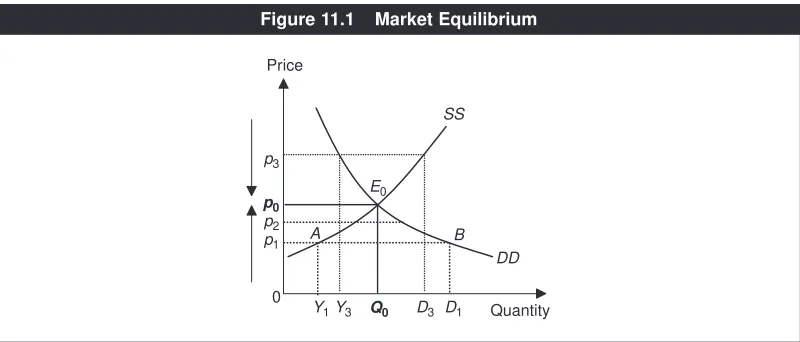
Consider the market for, say, ruled paper that you buy in stationery shops. Suppose these are available in one particular quality and you buy them by weight. Let the demand curve and the supply curve of this paper be DDand SS, as shown in Figure 11.1. The question is—what will be the price of this paper in the market and how much of it will be purchased and sold in the market?
Suppose that initially the price of this paper is p1. Notice that at this price the consumers are willing to buy the amount D1, while the producers are willing to supply the amount Y1. There is a mismatch. Consumers are demanding more than what the producers are supplying. The difference ABor Y1D1is the excess demand, defined generally as the excess of the quantity demanded over the quantity supplied.1 Will the price of paper remain stable at p
1? No. Excess demand will create competition among buyers to get hold of the limited amount available and this will raise the price. Suppose the price rises to p2. Will it be stable at p2? The answer is again no. The magnitude of excess demand is less than before, but it exists nevertheless, which will further push up the price. Indeed the
price will keep increasing as long as excess demand exists. The upward pointing arrow shows this. It is easy to see that this process of price adjustment will settle at p0, at which there is no excess demand.
Instead, if initially the price is above p0, say at p3, the producers are supplying more than what the consumers are willing to buy. There is excess supply, defined generally as the excess of quantity supplied over quantity demanded. It is equal to Y3D3. Excess supply generates competition among the sellers to sell the limited amount that the consumers are willing to purchase. This causes the price to fall. The process will continue until the price converges to p0at which there is no excess supply.
At p0then, there is market equilibrium, defined as the situation where excess demand or excess supply is zero. Put differently, market equilibrium occurs when quantity demanded and quantity supplied are equal to each other, or equivalently the demand and the supply curves intersect (at E0in the example). It is also called market clearing. The corresponding price is called the equilibrium price(p0in the example). The corresponding quantity demanded and supplied (Q0in the example) is the equilibrium quantity exchanged.
Furthermore, the fact that the price, irrespective of where it is initially, eventually settles at p0implies that the market equilibrium is stable.
Walrasian and Marshallian Stability
Note that the above argument of stability in analysing Figure 11.1 is based on the adjustment process that the price of a product adjusts upward or downward as there is excess demand or excess supply respectively. Stability of a market based on such a price adjustment process is called Walrasian stability, named after a 19th century French economist Leon Walras, who was the first to rigorously examine the issue of stability of market equilibrium via price adjustment.
D3 D1 SS Price
A
Quantity E0
0
Q0 p3
p2
DD B p1
Y1 p0
Y3
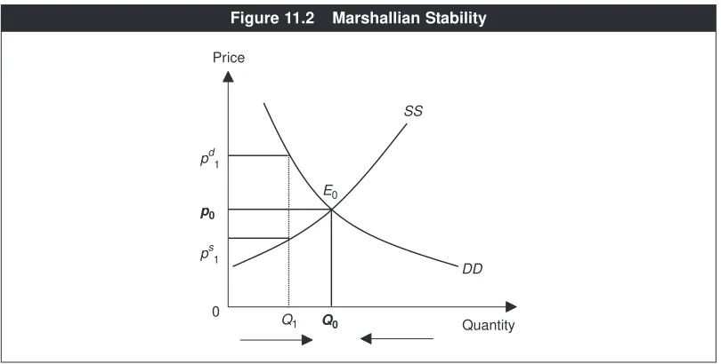
Alfred Marshall proposed a mechanism of market stability that is based on quantity adjustment, which goes by the name of Marshallian stability and is illustrated in Figure 11.2.
It has the same demand and supply curves as in Figure 11.1 but the stability argument proceeds in a different way. Suppose that at a given point in time, the quantity Q1is available in the market for exchange. The corresponding price on the demand curve is p1d, which can be interpreted as the ‘demand price’ in the sense that in order to purchase or demand Q1, the consumers are willing to pay p1d. Similarly, the corresponding price on the supply curve is p1s, the ‘supply price’— meaning that in order to supply the quantity Q1, the firms are willing to accept the price p1s.The Marshallian adjustment process states that the quantity will increase or decrease as the demand price exceeds or falls short respectively of the supply price. The underlying logic is that if, for example, consumers are willing to pay more (or less) than what the producers are willing to accept, more (or less) of the commodity will be available to the market by the suppliers.
At the quantity Q1, the demand price =p1dis greater than the supply price = p 1 s.
Thus, according to the Marshallian adjustment process, the quantity in the market will increase from Q1. The rightward pointing arrow indicates it. Where does this process lead to? The answer is Q0. The corresponding price, of course, is p0. The opposite happens but the quantity again converges to Q0, if initially the quantity in the market were greater than Q0. Therefore, the market equilibrium is stable under the Marshallian quantity adjustment too.
At a theoretical level, both adjustment processes seem reasonable. But there is not enough statistical evidence till today to tell us which one is more appropriate to assume. However, both processes lead to the same outcome in the case of a sin-gle market of the kind we are studying here. So, for us, it does not really matter.
SS Price
Quantity E0
0
Q0
DD pd1
ps1
Q1 p0
But, from now on, we will base our arguments on the Walrasian price mechanism and stability, which is more commonly used by economists and is somewhat more intuitive than the quantity adjustment mechanism.
Sustainable versus Non-sustainable Industry
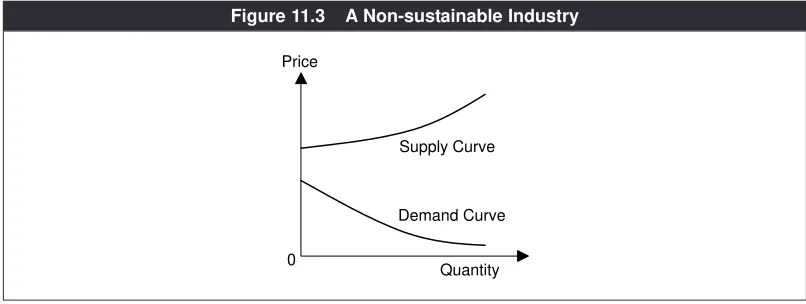
Figures 11.1 and 11.2 assume that the demand and supply curves intersect in the positive quadrant. Suppose that they do not, as in Figure 11.3. It does not mean that this can never happen or there is no equilibrium. It only means that the industry is not sustainable and the good is not produced, that is, the equilibrium production and consumption are zero because the cost is too high relative to what the con-sumers are willing to pay.2
However, it does not necessarily mean that the consumers cannot buy this product at all. If imports are allowed and the price of imports is low enough, then consumers can have it, although the domestic industry for the product is not sus-tainable and hence the domestic supply is zero. That is, the good is totally imported. For instance, at this point of writing, products like laser jet printers, computer memory chips, commercial jet planes and certain kinds of drugs are totally imported. Note the following.
(i) An industry may not be sustainable in one country, but sustainable in another.
(ii) Over time, a product, not sustainable earlier, can become sustainable in a country. For instance, colour TVs were not produced in India till the end of the seventies. In the eighties, the technology of producing colour TV became available in India and the market was large enough to start and sustain the colour TV industry.
2Put differently, the demand price is less than the supply price at any positive quantity sold. Supply Curve
Price
Quantity 0
Demand Curve
(iii) If a product becomes sustainable, it does not imply that we should not import any of it at all. Domestic production and imports can co-exist and benefit us.
Mathematically Speaking
Solving the Market Equilibrium
Suppose the demand and the supply functions are given respectively as qD=a−bp
and qS=c+gp, where a, b, g> 0 and a> c. Because band gare positive, the demand
function is downward sloping and the supply curve is upward sloping. The restriction a> censures that both curves intersect in the positive quadrant.
Market equilibrium is defined as qD=q
S, that is, quantity demanded equals the quantity supplied. Given the expressions of qDand qS, we then have
qD=q
S⇔a−bp = c +gp.
This is one equation with one variable, p. We can solve it and let the solution be denoted as p0. From the above equation,
This is the equilibrium price. Notice that if awere less than or equal to c, p0would have been negative or zero.
Given p0, we solve the equilibrium quantity, say Q0, by substituting the solution expression of p0into either the demand function or the supply function. Substi-tuting into the demand function,
We would obtain exactly the same expression of Q0if we substituted the expres-sion of p0into the supply function, c+gp.
* * * * * *
DEMAND AND SUPPLY SHIFTS
We now return to the situation where there is an equilibrium with a positive quan-tity exchanged. Our demand-supply ‘model’ can now be put to work in explaining various phenomena.
a bp a b a c b g
ag bc
b g Q
− = − −
+
= +
+ =
0 0
( )
.
p a c
b g
0 =
−
In reality, prices and quantities of products and services vary over time and space. A given piece of land that used to sell for Rs 1 lakh in Gurgaon district of Haryana 20 years ago may be selling now for Rs 50 lakh or even more. The South Indian delight dosa, of a particular kind and quantity may be selling for Rs 40 in Delhi, whereas in Chennai the same may be costing only Rs 5. Our demand-supply analysis helps us understand such phenomena among others.
Methodologically, either the demand curve or the supply curve (or both) can shift and as a result price and quantities change. Hence, we need to first under-stand how such shifts affect price and quantity.
Demand Shifts
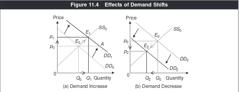
Turn to Figure 11.4(a). Initially, the demand and the supply curves are DD0and SS0respectively. They are drawn as straight lines just for graphical simplicity. The equilibrium point is E0, p0is the equilibrium price and Q0is the equilibrium quan-tity transacted. Suppose there is an increase in demand. Let DD1denote the new demand curve. We see that E1is the new market equilibrium point, p1is the new equilibrium price and Q1 the new equilibrium quantity. Hence an increase in demand raises price and quantity.
The ‘economic process’ behind these changes is the following. As demand increases (from DD0to DD1), at the original price (p0), there is excess demand (E0A). This tends to push up the market price. As a result, the new equilibrium price is higher. There is no change in supply or the supply curve and, because of a higher price, the producers move up along the (unchanged) supply curve and supply more to the market. Thus a higher quantity is sold in the new equilibrium.
Panel (b) of Figure 11.4 exhibits a decrease in demand and its effects. As the demand curve shifts to the left from DD0to DD2, at the original price, there is excess supply (equal to BE0). This pushes the price down. The producers move down along the supply curve. Consequently, the equilibrium price and the equilibrium quantity
Quantity
transacted both fall. The price and quantity at the new equilibrium are p2and Q2
respectively.
Supply Shifts
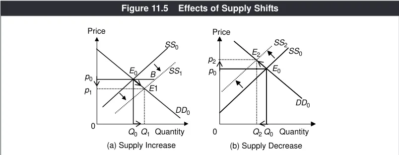
These are shown in Figure 11.5. In panel (a), there is an increase in supply (from
SS0to SS1). At the original price, this creates an excess supply (E0B). The price is pushed down. There is no change in the demand curve. As the price falls, the con-sumers move down and to the right on their demand curve. In summary, the price falls (from p0to p1) and the quantity increases (from Q0to Q1).
Panel (b) of Figure 11.5 demonstrates a decrease in supply. The supply curve shifts to the left from SS0to SS2. Initially a decrease in supply causes an excess demand. The price rises. Consumers move up on the demand curve and buy less. These implications are the opposite of those of an increase in supply.
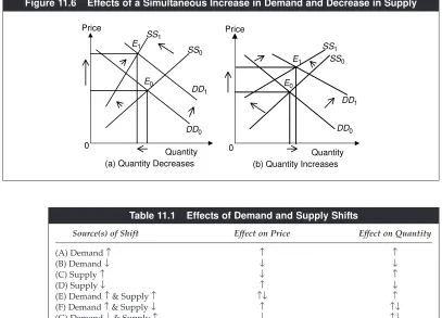
Simultaneous Shifts
It is possible that both curves shift at the same time. The net impact is then the sum of the two individual impacts. For instance, in both panels of Figure 11.6, the demand increases and the supply decreases. Individually, both these shifts tend to increase the price and, therefore, the market price increases unambigu-ously. However, an increase in demand tends to increase the equilibrium quan-tity, while a decrease in supply tends to decrease the equilibrium quantity. Thus the net impact of these two shifts on the quantity is ambiguous, depending on the relative magnitude of the two shifts. In panel (a), the demand-shift effect is less and the equilibrium quantity is less. In panel (b), the demand-shift effect is more than the supply-shift effect and, thus, there is an increase in the equilib-rium quantity available in the market.
Quantity
You can similarly work out the effects of other joint shifts. Various outcomes are summarised in Table 11.1.
We now examine the effects of various sources of demand and supply shifts by considering one at a time.
Sources of Demand Shift
In Chapter 2, we learnt that the demand curve shifts if, for instance, income and prices of related goods change. We will consider some of these shifts.
Suppose the total income of consumers in the market increases. If the good is normal, the market demand curve will shift to the right. In this case, row (A) in Table 11.1 applies. The equilibrium price will increase and more quantity will be available in the market. If the good is inferior, row (B) applies. The effects are opposite—price and quantity will both decrease.
As a real-life example, in the nineties, the prices of flats and land in many cities in Kerala sky-rocketed. Why? Because, many Keralites went to the Middle East
Quantity
(b) Quantity Increases Price
(a) Quantity Decreases
0 Price
0
E0 E1
SS1
Quantity E0
DD0 SS0 E1
DD1 SS0
SS1
DD0 DD1
Figure 11.6 Effects of a Simultaneous Increase in Demand and Decrease in Supply
Table 11.1 Effects of Demand and Supply Shifts
Source(s) of Shift Effect on Price Effect on Quantity
(A) Demand ↑ ↑ ↑
(B) Demand ↓ ↓ ↓
(C) Supply ↑ ↓ ↑
(D) Supply ↓ ↑ ↓
(E) Demand ↑& Supply ↑ ↑↓ ↑
(F) Demand ↑& Supply ↓ ↑ ↑↓
(G) Demand ↓& Supply ↑ ↓ ↑↓
for work and sent back their money to buy real estate. There was a major increase in the income of people in that region. Real estate is obviously not an inferior good. As our demand-supply ‘model’ predicts, its price increased substantially.
Similarly if the price of a substitute good increases, the demand curve of the good in question will shift to the right. In this case, row (A) in Table 11.1 applies. Price and quantity will increase. For instance, if coffee becomes more expensive for some reason, people will switch to tea. The demand curve for tea will shift out-ward. The price of tea will increase and more of tea will be sold in the market. In fact, this happened in the world market of tea in the late nineties. Brazil is the biggest producer of coffee in the world market. In the mid-nineties, the coffee production in Brazil was severely curtailed by bad weather. The coffee prices in the world market increased substantially and remained higher than before for a few years. It was observed that during the same years, the tea prices also went up in the world market without any major problems in the production of tea as such.
On the other hand, if the price of a complementary good rises, the demand curve shifts to the left; (B) in Table 11.1 applies here and both price and quantity fall.
If peoples’ taste for a product improves (or deteriorates), the demand curve shifts to the right (or left). As a result, the price and the quantity both increase (or decrease) in the market. As a hypothetical example, suppose that medical research shows that eating 200 gm of moong dala day significantly improves memory. This will surely increase the demand for moong dalby many consumers. You will soon observe that moong dalis costlier and more of it is sold in the market. As a real-life example, the demand for air travel plummeted right after 11 September 2001, which was because of the fear of terrorism and can be interpreted as a change in taste for air travel. As a consequence, the price of airline tickets within the US went down considerably and there were much fewer scheduled flights.
Even if the individual demand curves remain the same, the market demand curve can shift if the number of consuming households changes. An increase (or a decrease) in the number of consumers in the market will shift the market demand curve to the right (or left). As a result, price and quantity both will increase (or decrease). As an example, in the eighties, Delhi witnessed a surge in the price of land. It occurred because many people migrated from Punjab to Delhi, follow-ing disturbances in Punjab, and this shifted the market demand curve for real estate in Delhi.
Sources of Supply Shift
time. A particular chip becomes obsolete after a few years. Another example is photograph printing. By the end of 2002, in Delhi, an instant photograph (by Polaroid technology) cost around Rs 120 for 8 copies. By the end of 2004, due to digital photography and the facility of printing from computer files on glossy paper, it cost Rs 100 for 25 copies.
In Chapter 3, we also learnt that increases in input prices shift the supply curve to the left. In such a situation, as shown in row (D) of Table 11.1, the price rises and the quantity sold falls. The opposite happens if input prices fall. Desktop com-puters are a good example. They have inputs like memory chips and mother-boards and the prices of these inputs are falling over time. Thus, a computer with same configurations and quality is becoming cheaper over time.
As another example, between 2004 and 2005, the crude oil price in the world market soared. In the US, it led the average retail petrol price to increase from $1.87 per gallon in September 2004 to $2.90 in September 2005, a 55 per cent increase. Petrol is used as an input in many businesses, which typically involve transport. In October 2005, FedEx, the premier courier service company announced that it would increase its air shipment rates by 3.5 per cent.
An increase or a decrease in business taxes works in a similiar manner as an increase or a decrease in an input price. For an application of how the price of a service is affected by input prices and taxes, see Clip 11.1.
Clip 11.1: ‘Unfair Air Fare’
On 13 October 2004, Hindustan Times ran an article by the title: ‘Unfair Air
Fare’. The main point was that air fares in India are very high compared to rates outside—in some cases about three times as high. For example, based on 21 days advance ticket booking, a one-way flight from Delhi to Trivandrum cost Rs 13,120 and the flying time was two hours and 45 minutes. In compar-ison, a Delhi to Singapore flight cost Rs 15,750 one-way and the flying time was five hours and 30 minutes.
While the airlines blamed the high fares on fuel prices, the article argued that flawed policy and ‘back-breaking’ taxes were also significant factors. For instance, because of government policy on fuel prices, the Air Turbine Fuel (ATF) rates in India were about two and a half times more than elsewhere. In Singapore, one kilolitre of ATF cost Rs 15,100, whereas in India it cost Rs 30,000. There was also 8 per cent excise tax and sales taxes ranged from 4 to 29 per cent in different states. Furthermore, navigation charges and land-ing fees constituted about 30 per cent of operatland-ing costs whereas in other countries they were about 15 per cent of operating costs.
We also learnt in Chapter 3 that an increase or a decrease in the expected future price of a product may motivate sellers to hoard and flood the market with their goods in the current period. In other words, as the price of a product in the future is expected to decrease or increase, the current supply curve will shift to the right or to the left with the result that the current price will decrease or increase.
As a prime example, think of stocks of various companies, which are sold in the share market—pretty much like other commodities. Investors’ expectations play a big role in determining a stock price. If an investor speculates that the price of a stock that he is holding is to going to double or halve in the next few weeks, he is going to buy more of this stock or sell off some of it respectively. If many investors think the same way, it will impact the stock market today—irrespective of whether their expectations turn out to be correct in the future. As an example, on Monday, 17 May 2004, the ‘Sensex’, an index of selected stocks in the Indian stock market, fell precipitously by 565 points (11 per cent). This was completely unprecedented in the history of the Bombay Stock Exchange. Why? It was because the UPA registered an unexpected win in the general elections at that time. This led many important investors to think that the country may roll back the reforms, which would adversely affect business, profits and the stock prices in the future. Thus there was a decrease in the expected future prices of stocks. The investors sold their stocks in huge volumes, which resulted in a huge drop in the stock prices across the board. Some people have called this day the ‘Black Monday’ of the Indian stock market.
A change in the number of firms affects the market supply curve too. An increase in the number of firms, for example, would shift the market supply curve to the right. As a result, the price will fall and a higher quantity will be sold. In common language this is the case of an increase in competition.The
telecommu-nication market is a good example. In the early nineties, MTNL (Mahanagar Telephone Nigam Limited) was the sole provider of the ISD facility in Delhi. An ISD call from India to America cost over Rs 50 per minute. Between 2004 and 2005, there were other land-line providers like Tata-Indicom, Reliance and Touchtel, which charged less than Rs 10 per minute.
ANALYTICAL APPLICATIONS
The demand-supply analysis is not only helpful in understanding what happens in some isolated markets but also has broader applications. We can use it to analyse how economic policies affect markets; how the exchange rate between different currencies may be determined; and even how catastrophes like famines occur. In what follows, we consider three applications in different areas of economics.
Application A: Burden of a Sales or a Service Tax
store, which has a big collection of leather jackets of very good quality. You are a person who cannot compromise on quality. Although you know that there are other shops selling leather jackets, you are unsure of their quality. So this is the only store for you. Imagine that you do find a jacket that you really want to have and it has a price tag of Rs 2,699. Not only is it within your budget but you will also have Rs 301 left in your pocket to spend on other enjoyments. You think of spending this left-over money on food at your favourite restaurant with your friends in the evening. With your jacket in hand, you walk to the check-out counter in the store and the sales person tells you (with a smiling face) that the bill comes to Rs 2,968 and 90 paise. You are jolted but are politely told that there is a sales tax of 10 per cent, which you have to pay as the consumer and so the total comes to this amount. You have no choice and you buy the jacket. You are happy about the jacket, of course, but your mood is spoiled. You wonder (and despair) why you, the consumer, have to pay this tax instead of the seller.
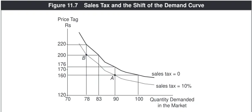
Take it easy. Indirectly, the producer is also sharing the tax burden partly and this is what this application is all about. Consider Figure 11.7. The heavy line is the market demand curve for a product when the sales tax is zero. As an illustration, four price-quantity combinations are shown. Note that, since there is no sales tax, whatever price is written on the sales tag is the price the consumers pay.
Now suppose that the state government levies a sales tax of 10 per cent. Will the demand curve remain the same? No. For instance, previously, at price Rs 160, the consumers were buying 100 units. How many will they buy now? Note that, with a 10 per cent sales tax, a price tag of Rs 160 actually means Rs 176 for the consumer (Rs 160 plus 10 per cent of it). So, at the price tag of Rs 160, the consumers will buy whatever they would have bought at Rs 176 without the sales tax. The answer from the graph is 90 units. Thus, the corresponding point A(with the price tag equal to
Rs 160 and the quantity demanded equal to 90) is on the new demand curve.
120 170 220
70 100
160 176
90 78 83
sales tax = 0 sales tax = 10% 200
A B
Price Tag Rs
Similarly, at a price tag of Rs 200, the consumers were previously buying 83 units. Now in the presence of a 10 per cent sales tax, the same price tag means Rs 220 for a consumer. Hence, the quantity demanded will be equal to whatever the con-sumers would have bought at Rs 220 without any tax, that is, 78 units. Point Bis on the new demand curve. If we join points like Aand B, we get the new demand curve, which is shown as the thin line.
Two important points need to be noted. (i) The vertical distance between the old demand curve and the new one is the sales tax paid. For instance, at the quan-tity purchased equal to 90, the difference is Rs 16, which is 10 per cent of Rs 160. Similarly, at the quantity = 78, the difference is Rs 20, which is 20 per cent of Rs 200. (ii) At each quantity sold, the corresponding point on the old demand curve measures the consumer price—the price that the consumers actually pay, inclusive of the tax. The corresponding point on the new demand is the producer price—the price that the producers receive. The difference is the tax per unit which goes to the government.
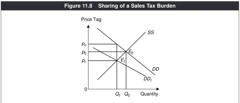
Once these points are understood, the rest of the analysis is straightforward. Turn to Figure 11.8 depicting the market for any particular good. The supply curve is denoted by SS. The demand curve without any sales tax is DD. The point E0marks the market equilibrium; p0is the equilibrium price, same as the consumer and the producer price. This is the starting situation.
Suppose the government imposes a sales tax. This vertically shifts the demand curve down. Let DDt be the new demand curve, intersecting the supply curve at Et.The new equilibrium price is pt and the new amount sold is Qt, less than what was produced and sold before. From point (ii) above, pt(on the new demand curve) is the producer price and pc (on the old demand curve) is the consumer price. The distance ptpcis the sales tax per unit, paid to the government.
Compare this with the old equilibrium price p0. How much more are the consumers paying? It is pcp0. This is the burden of the sales tax on them. The not-so-obvious point is that the producers are taking a price cut, p0pt, as they were
SS
Q0 Qt
DDt DD
0
Et
Quantity Price Tag
pc
E0
pt p0
receiving the price p0before and are now receiving pt. Hence, p0ptis the tax burden on the producers. The sum of the tax burdens is equal to pcp0+p0pt=pcpt, the tax per unit accruing to the government. In other words, not just the consumers but also the producers share the sales tax burden, although the tax is levied on the consumers. Of the total burden, the shares are pcp0/pcptand p0pt/pcptfor the con-sumers and the producers respectively.
The economics behind both parties sharing the tax burden is as follows. A sales tax, by lowering the demand curve, lowers the base price (or the price tag) of the product. This means that, for the consumers, the new price is less than the old price plus the tax, that is, they do not bear the full burden of the tax. The very fact that the base price falls means that the producers are also sharing the burden.
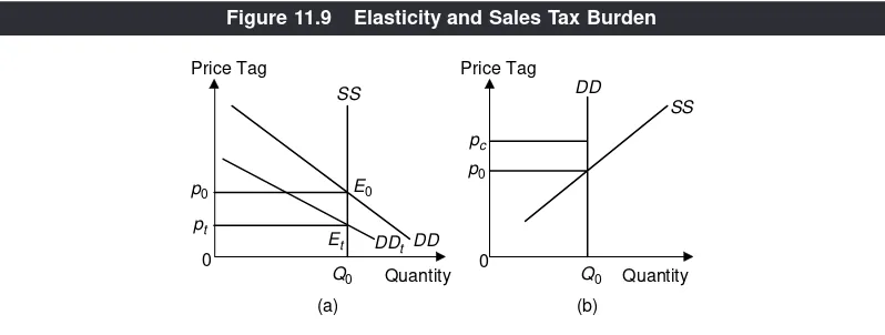
What factors determine who shares how much. It is the elasticity of demand and supply. To see this, turn to Figure 11.9. The two panels show two extreme ations. In panel (a), the vertical supply curve has zero price elasticity. In this situ-ation, as the sales tax is levied, ptis the producer price but the consumer price is same as the original price p0. Hence, there is no price increase for the consumers. It is thus the producers who share the full burden of the tax. The economic intu-ition is that the producers cannot adjust at all and are hence forced by the market to take the full burden of the tax, although legally or technically the tax is paid by the consumers (as it appears on the receipt).
On the other hand, panel (b) depicts a vertical demand curve having zero price elasticity of demand. In this case, there is no shift of the demand curve, since the consumers have topurchase Q0. Of course, the supply curve does not shift. This implies that there is no change in the price tag or the producer price. Thus, producers do not share any burden of the tax. The consumers pay p0plus the tax, marked by pc. They share the full burden. Why? Because they cannot adjust their demand for the product at all. It is the opposite of the situation illustrated in panel (a).
Combining the reasoning in the two extreme cases, it follows that if the sup-ply curve is normal and upward-sloping and the demand curve is normal and
SS
downward sloping, then both parties must share the burden, as shown earlier in Figure 11.8.
Moreover, the pattern of burden-sharing in the extreme cases illustrates that who shares how much depends on the elasticities: the higher the elasticity of demand (or supply) relative to supply (or demand), the higher is the share of the burden by producers (or consumers).
Note that the service tax works the same way. It is a tax to be paid by the consumer for a service. Yet the producer will also indirectly bear a part of this tax burden unless his supply curve is perfectly elastic.
Application B: Exchange Rate Determination
International commerce involves the exchange of currencies. Different exchange rates between different currencies prevail in the currency market. For example, on 30 June 2004, the exchange rate between US dollar and Indian rupees was Rs 45.99 per dollar. On the same day, the exchange rate was $1.81 = £1, between US dollar and British pound. The exchange rate between a given pair of currencies changes over time too. Compared to the dollar-rupee exchange rate on 30 June 2004, on 31 March 2005, it was $1 = Rs 43.62.3
Variations in the exchange rate can be understood by the demand-supply analysis also—once you realise that the exchange rate is simply the price of one currency in terms of another. When we say, for example, that $1 = Rs 46, it means that if you sell or buy one dollar, you get or have to give Rs 46, that is, the price of one dollar in terms of rupees is Rs 46.4Equivalently, the price of a rupee in terms of dollars is $ 1/46. Note that it does not matter whether we talk about the price of dollars in terms of rupees or the price of rupees in terms of dollars because, by definition, one is the inverse of the other. So let us stick to the term ‘price of dollars in terms of rupees’ as the exchange rate between the two currencies. The question is—how is this price determined in the market for currencies?
Just like the price of a banana is determined by the demand and supply of bananas, in the currency market the price of dollar is determined by the demand and supply of dollars (in exchange for rupees). In the context of commerce between India and the US, who demands dollars? It is the Indian importers of American goods and services. For instance, you want to do a master’s in the US, for which there are application fees charged by American universities. They would want their fees in dollars, so you would have to demand dollars and pay them in dollars. How does it work? You go to a bank, apply for dollars, deposit your rupees and the bank gives you a draft in dollars in the names of the respec-tive universities. Indirectly, the bank is placing your request (demand) for dollars
3See the web publication by the Federal Reserve Bank of the United States, http://www.federalreserve.gov/releases/
H10/hist/
through its correspondent bank, which is authorised to deal with foreign currency directly.5
The point is that, given the price of dollar, Indians (through their representative banks) demand a certain amount of dollars in the currency market—this demand originates from our desire to import goods, services and assets from the US. For instance, if an Indian company wants to acquire a company in the US, it has to demand dollars because the owners of the selling company would want their pay-ment in dollars and not in rupees.
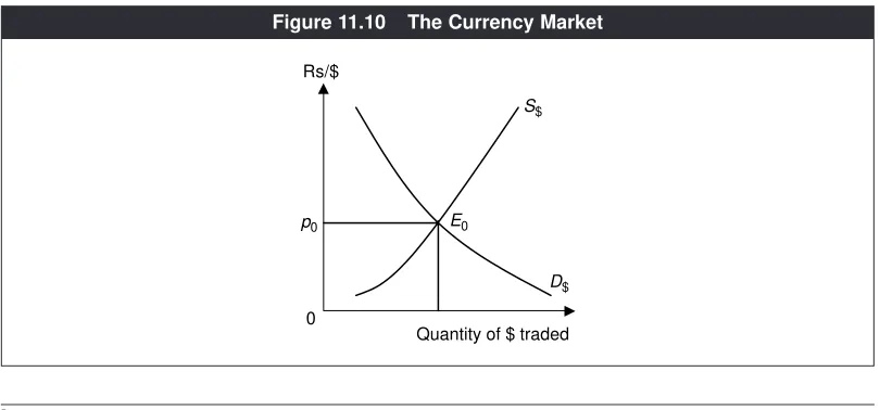
This implies that if the price of dollar changes (that is, if there is a change in the exchange rate), our demand for dollars will change. To continue with the example of applying to US universities, if, hypothetically, the exchange rate falls from $1 = Rs 46 to $1 = Rs 16 only, it is almost a certainty that the applications from India to do a master’s will increase. This means that a decrease in the price of dollars will increase the demand for dollars. Hence, there is a normal, down-ward sloping demand curve for dollars. This is shown in Figure 11.10 by the D
$
curve.
Consider who would supply dollars into the currency market. It is the American importers of Indian goods, services and assets. If Bill Gates wants to buy a flat in Bangalore he would, through his bank, have to supply dollars to the currency market, get rupees in exchange and pay the Indian owner of the flat in rupees.6In general, how would an increase in the price of dollar affect the
‘quan-tity supplied of dollars’ (in exchange for rupees)?
This is a bit tricky. If the American import demand for Indian goods is absolutely inelastic, they would have to pay or supply less dollars because one dollar is now fetching more rupees and hence for the same good priced in rupees,
5In the process, of course, the bank is charging you a service fee. But we can ignore it for analytical convenience. 6If the flat is priced at, say, 1 crore and the current exchange rate is, say, $1= Rs 50, he would have to supply $1 crore/50 =
$2,00,000 to the currency market.
S$
E0 Rs/$
Quantity of $ traded D$
0 p0
they would have to pay less in dollars. Then, the quantity supplied of dollars will decrease in the currency market. On the other hand, if their demand for Indian goods is highly elastic, cheaper Indian goods will generate a huge increase in their import demand for Indian goods and as a result they will end up supplying more dollars to the currency market. Thus, whether the total supply of dollars will increase or decrease depends on the price elasticity of import demand for Indian goods by the Americans. If we apply the relationship between a price change and the total expenditure on a product as studied in Chapter 2, it follows that the total supply of dollars (foreign currency) will increase or decrease as the price of dollar increases according as the foreign import demand for domestic goods is greater or less than one respectively. For expositional simplicity, we will assume here that this elasticity is greater than one. This then implies that the total supply of dollars will increase with the price of dollar. Figure 11.10 shows an upward sloping sup-ply curve of dollar, S$.
The intersection of the D$curve and the S$curve determines the price of dollar or the exchange rate. In Figure 11.10, the equilibrium in the foreign currency mar-ket is at E0. The equilibrium price is p0. If p0happens to be 45, then the market exchange rate is $1 = Rs 45; if p0= 50, then the market exchange rate is $1 = Rs 50; and so on. This is how the exchange rate between two currencies is determined by the forces of demand and supply.
The demand-supply framework can be applied to understand what factors affect the exchange rate and how. Let us take an example. Suppose, within a given period, the Indian economy experiences an inflation rate of only 5 per cent, while in the US economy it is 12 per cent. All other things remaining unchanged, this would mean that American goods will be costlier relative to Indian goods. As a result, we would like to demand less of American goods and Americans would like to demand more of Indian goods. In turn, this will mean that we would like to demand less of dollars in the currency market and Americans would like to supply more of dollars. The D$curve will shift to the left and the S$curve to the right. The price of dollar will fall—one dollar will command less rupees or one rupee will command more dollars.
Hence, as a result of US inflation being higher than inflation in India, the rupee will be stronger, that is, it will appreciateand the dollar will be weaker, that is, it will depreciatein the currency market.
Application C: Explaining Famines
Famines have terrible consequences—millions of people die of starvation and dis-eases. Although these are less frequent now than they were, say, hundred years ago, they nevertheless occur in modern times, the Sudanese famine in 1998 being the most recent.7In what follows, we will illustrate the research (work) on famine by Amartya Sen, a Nobel laureate in economics.
The standard notion is that a famine occurs due to a drastic shortfall of food grain production and supply for some reason, for example, a severe drought or a massive flood. Sen calls this the FAD theory of famine, where FAD stands for ‘food availability decline’. His ‘thesis’ is that not all famines are due to FAD. A famine may be ‘man-made’. A large section of the population of the poor in a region can be deprived of food, even when there is no decline in the total supply of food.
We can understand famines by analysing demand and supply forces. We will first outline the FAD theory and then follow it by a discussion of Sen’s theory of famines (1981).8
THE FAD THEORY
A famine occurs in the form of epidemics and deaths from pervasive starvation. In turn, starvation, that is, deprivation from basic food items is reflected mostly in terms of the staple food of the region. Hence, with regard to the question of what causes a famine, we can limit ourselves to examining how a large section of a region’s population is not be able to obtain the minimum amount of staple food for survival. Let us call this staple food rice.
Now turn to Figure 11.11, which depicts the individual and market demand curves for rice as well as the market supply curve of rice. Let us say that there are three families, A, B and C, in the market. The panels (a), (b)and (c) graph the demand curves of these families respectively. The B-type family’s demand curve lies to the right of that of the A-type and the C-type family’s demand curve lies to the right of that of the B-type. We can interpret the A-type as the poorest, the B-type as the next poorest and the C-type as the richest.
See that when the price of rice is p1, the A-type family cannot afford to buy any rice at all, but the B-type or the C-type can. As shown, this price is above the pointa– at which the DDAcurve intersects the price axis. Hence, the A-type family’s quantity demanded is zero. This is not true for the B-type or the C-type family. The former
8There is no claim on the originality of the ideas, but the demand-supply exposition is a result of the author’s own work.
For Sen’s theory of famines, see: Sen, Amartya. 1981. Poverty and Famines: An Essay on Entitlement and Deprivation.: Oxford University Press.
demands the amount B1and the latter the amount C1. If the market price is p2, the A and B-type families cannot buy rice but the C-type can; its quantity demanded is C2.9The rightmost panel depicts the market demand curve, DD
M, as the horizontal
summation of the three individual demand curves.
This graph assumes that there is one family of each type. But it is not restric-tive. If there are more families of any given type, the market demand curve is obtained by horizontally summing up the demand curves of all the families. The resulting curve will look similar to DDM.
From the supply side, let, initially, the total available amount be M0. It is drawn vertically to represent that after the harvest, this is the total, potential amount available for consumption.10The equilibrium price is then p
0. At this price, all fam-ilies are able to buy rice. The types A, B and C respectively buy A0,B0and C0. This situation can be interpreted as one in which there is no starvation or famine.
Now suppose that (for some reason) there is less total amount available, equal to M1. The equilibrium price is higher, equal to p1. Notice that at this price, the poor-est cannot afford to buy any rice, but the other types can. We can think of this situ-ation as ‘starvsitu-ation’—some people at the lower income levels just cannot afford to buy enough food for survival. If, instead, the total available amount were much less compared to the initial situation, for example, equal to M2, the price would have risen to p2and both A-type and B-type families would have been driven out of the market. We can interpret this as a situation of famine or massive starvation. Whether exactly two types of families are deprived of the staple food or not is immaterial. This situation generally represents that a large number of people are under starvation. This is the FAD theory. In summary, it says that a drastic fall in the total availability of food can raise the price of the staple food to such an extent that many families at the lower end of income levels may no longer be able to afford to buy the minimum amount needed for a healthy survival. Consequently, massive starvation and famine may follow.
SEN’S THEORY
Sen argued and emphasised that a famine could be an income distribution prob-lem,meaning that if the distribution of income becomes so unequal that a large section of a region’s population becomes relatively much poorer than before, they can no longer afford to buy a minimal amount of food even when there is no decline in the total availability of food.Sen went on to argue convincingly that this was indeed the case in the Bengal famine of 1943–44, which claimed the lives of 3 lakh people.
How can it be that when there is no decrease in food availability, a large number of people cannot buy the minimum amount of staple food for survival?
9If the price of rice is p
The key is that, the supply remaining unchanged, if the demand for the staple food by people who are not poor increases sufficiently, it can drive the poor fam-ilies out of the market and force them to starve.
Turn to Figure 11.12, which is similar to Figure 11.11. Suppose that starting from the situation where p0 is the equilibrium price and every family is able to buy some rice, the demand curve for rice by the C-type increases from DDCto DD’C. Note that the market demand curve shifts to DD’M. As a result, the equilibrium price increases to p1and the A-type family cannot afford to buy anything. The same reasoning implies that if the C-type’s demand curve had increased more, the price increase would have been greater and even the B-type could have been thrown out of the market. The whole point is that if the demand for the staple food by the non-poor increases sufficiently—because the non-poor become even richer—the price would rise sufficiently so that a large number of people in the poor classes are unable to buy the minimal amount of the staple food and hence a famine occurs.
Note that there is no decline in the total availability of food. But, because of demand pressures from one class of people, this class is able to claim a large share of food via the market mechanism at the expense of the remaining people. This is the gist of Sen’s distribution theory of famine.11
PRICE MECHANISM—THE INVISIBLE HAND
The purpose of laying down the above applications is to drive home the point that the reach of the demand-supply analysis is long. Many important problems
b
Figure 11.12 Sen’s Distribution Theory of Famines
11In establishing that this was the nature of the Bengal famine, Sen first provided data (statistics) to show that a decrease
in economics can indeed be meaningfully studied and understood using this analysis.
All through these examples, we have seen how demand and supply curves shift and how they affect prices and quantities in a market economy. Such shifts occur not just in a few selected markets but in almost all markets and almost always over time. The beauty is that there is no central or supreme planning authority that has to coordinate the actions of innumerable consumers and producers in the market. A change in the behaviour of one group—either producers or consumers—gets reflected in a price change, which acts a signal to the other party and both parties adjust in the end in a mutually consistent way. This is called price mechanism. Adam Smith, considered the father of economics, compared price mechanism to an ‘invisible hand’ and held that the behaviour of the consumers and the producers is coordinated in a market economy by an invisible hand.
A fundamental question is whether such free working of the price mechanism or the free operation of a market serves a society the best. The answer is ‘not always.’ As a glaring example, we saw that a catastrophe like a famine can occur in a market economy. There are other less extreme situations where a free market may not work in an ideal fashion. In such situations, there is a justified role for the government to intervene in the market in some desirable way. A systematic analysis of situations where a free market may fail to act in the society’s best interest and of the best corrective forms of policy intervention will be taken up in Chapter 12.
In what follows, we take as granted that as a matter of practice, governments do intervene in the markets and we will study the implications of such inter-ventions.
GOVERNMENT POLICY IN A MARKET
A government can interfere in a market in a variety of ways.
(a) It can levy taxes or grant subsidies to either consumers or producers or both.
(b) It can control prices in the form of ration and support prices.
(c) It can regulate entry into a market through an exclusive licensing system
and other requirements (or what is called licence raj).
(d) It can regulate mergers and acquisitions of companies and the pricing
policy of firms (different from controlling the price itself).
(e) It can choose to do the business itself as a public sector firm (for example
in the steel and civil aviation sectors) or in services like electricity and telecommunication.
Business Taxes and Subsidies
Levying taxes and granting subsidies on commodities and services are called indirect interventionsin the sense that these policies are not meant to forcefully ensure a particular price or particular quantity that the government believes to be right for the society. Rather the end is achieved indirectly by influencing the price and that is why these are called indirect interventions. In many cases, indirect taxes are levied for revenue purposes only.
We have already discussed the effect of sales or service taxes—the consumer price increases, the producer price falls and, therefore, both parties share the burden of this tax, although it is the consumers who pay this tax directly to the government. Exactly in the same way, taxes that are directly paid by the producers, for exam-ple, an excise duty or a VAT, are borne by producers and consumers both. Who shares how much is dependent on the price elasticity of demand and supply as in the case of sales tax.
While we have focussed on taxes that reduce the produced and consumed, in certain markets the government encourages production and consumption by granting subsidies. For instance, through nationalised banks, the government pro-vides subsidised loans to small businesses in rural areas.
Control Price and Support Price
As we shall see, these are prices set directly by the government in certain markets and hence called direct interventions.
CONTROL PRICE
For necessary food items like rice and wheat, it is felt that if the prices are totally left to the free market, the poor and the needy may not be able to afford them. The government sets a low price and the products are sold in the ration or ‘fair price’ shops. This is illustrated in Figure 11.13(a). Suppose the demand and the supply curves in this figure refer to wheat. If there are no interventions, the free market price of wheat will be p0and the quantity Q0of wheat will be produced and sold. If it is presumed that the price p0is too high for the poor, the government would step in and set a price below p0, say p1. This is a situation of control price. What are the implications?
There is a further implication. Because of the shortage, some people will always want to pay a higher price in order to obtain more than the ‘rationed’ amount. Thus the ration-shop licence holders have an incentive to illegally sell at a higher price though back door means. In other words, a price control programme invari-ably begets a black market, which otherwise would not exist.12
In India, there were about 4.77 lakh ration shops as of 2004. They come under what is called the ‘public distribution system’ or PDS, which has recently evolved into TPDS, ‘targeted public distribution system’. PDS or TPDS is instituted by the central government. See Clip 11.2 for a brief account of the PDS/TPDS.
12The same is true in currency markets. When currency rates are artificially set different from the equilibrium rates, hawala
markets emerge.
Clip 11.2: PDS/TPDS in India
The public distribution system (PDS) came into existence during World War II. Through this the government sells grains, mostly rice and wheat. (Other products like sugar and edible oil used to be included on a limited scale.) Through the Food Corporation of India (FCI), the government procures grain at a procurement price and stores them. In distributing the grains across the country for consumption, the central government first provides the states and union territories these commodities at ‘central issue prices’ (CIPs). In turn, the states and union territories fix the end retail price by taking into account the margin for wholesalers, transportation costs, local taxes and so on.
Price Price
Quantity Quantity
D S
D
S
p0
S1
Q0 D1
D2
p1
S2 p2
(a) Control Price (b) Support Price p0
Figure 11.13 Control Price and Support Price
Control price programmes do not just exist for food grains. Rental markets in metropolitan areas like Chennai, Delhi, Kolkata and Mumbai are other prime examples. There are rent control acts for each of these cities. Essentially, these acts have frozen the rent for a large number of urban properties over several decades. At current prices, the controlled rents are ridiculously below their market rates— in some cases even less than 1000th fraction of the market rates. An account of the implications of such acts is given in Clip 11.3.
Historically, the primary objectives of the PDS have been to ensure price stability of food grains and provide the poor an access to basic food at rea-sonable prices. Till 1997, the access to the PDS (ration shops) did not depend on the household income. Virtually anyone having a permanent address could obtain a ration card. In 1997, PDS became a targeted PDS (TPDS), meant to target the poor families. The TPDS was initially a two-tier subsidy system—one for the poor below the poverty line (as defined by the Planning Commission for different states in 1993–94) and the other for the poor above the poverty line. In 2000–2001, Antyodaya Anna Yojana was initiated to tar-get the poorest among those who were below the poverty line. Hence, as of now, it is a three-tier subsidy system. Accordingly, there are CIPs for each grain (rice or wheat). For instance, in 2000–2001, for the poorest of the poor, the end-retail prices were Rs 2/kg for wheat and Rs 3/kg for rice. For the rest below the poverty line, these are Rs 4.15/kg for wheat and Rs 5.65/kg for rice. For those above the poverty line and yet relatively poor, these prices are Rs 6.10/kg for wheat and Rs 8.30/kg for rice (which are at par with the government’s cost). The state governments shoulder the responsibility of identifying the poor.
How far has the PDS or the TPDS reached the poor? In 1999–2000, 36 per cent of the below-poverty-line households and 31 per cent of the poor but above the poverty line reported purchasing rice or wheat from the PDS. Various case-studies point to a number of reasons for the relatively low par-ticipation rate of the poor—like the difficulty in obtaining ration cards, uncer-tain ration supplies and inferior quality of PDS grains. Furthermore, there is also fraudulent or illegal diversion of grains from the PDS—consistent with the black-market implications of a ration system. According to Ramaswami (2007), the future of the food subsidy programme may not lie in a centralised PDS but in a regionally differentiated one. Another option could be food coupons or food stamps, where food is supplied by the private sector.
Reference
SUPPORT PRICE
While some consumers of certain food grains are offered a price control programme, growers of various food grains are offered a price support pro-gramme by the government. That is, the government guarantees them a price higherthan the market price. This is called a support priceor a minimum support price (MSP). For instance, for common paddy, during the kharif market season (September–October) of the financial year 2003–2004, the MSP was Rs 550 per quintal. During the rabimarket season of 2002–2003, it was Rs 620 per quintal for wheat.
What is the rationale for the support price? It is thought that since farmers are poor, price fluctuations resulting from the operation of free markets may hurt their well-being, especially if the prices become very low. Therefore, a minimum support
Clip 11.3: Some Implications of Rent Control Acts
Not only are rents abysmally low but also it is very hard under the law to remove a tenant. For instance, in Delhi, to remove a tenant, the landlord has to prove, among other things, that he/she has no other place to live. But the landlord would be living somewhere else; perhaps he/she has some other property; hence it is difficult—almost impossible—to establish that one has no other place to live.
What are the implications? There is no incentive for property owners to maintain the rental property in terms of quality other than what is (legally) required for some bare minimum level (for example, providing electricity and water connections). The renters have absolutely no incentive to vacate. If they die, according to the law, the rental property is automatically inherited by their children. Who does not want some space in an urban area, which is almost free of cost? If the landlord really wants to get some tenant out, so that he/she can use the property, typically and illegally, the tenant is paid a huge sum of money. Consider the fairness of all this—to reclaim your own property, you have to pay somebody else! Another way to remove a tenant is to use threat and violence.
Interestingly, according to Suketu Mehta in his best seller, Maximum City: Bombay Lost and Found, a majority of police complaints and crimes (taking small and big occurrences together) in Mumbai owe their origin to the Bombay Rent Control Act! That is, violence and crime are by-products of con-trol price regimes too.
Clip 11.4: The MSP Programme in India
India has an elaborate MSP programme since the sixties. Currently the central government announces MSPs for 24 major crops. Typically, MSPs are announced each year by taking into consideration the recommendations by the CACP (Commission for Agricultural Costs and Prices). Several factors go into the MSP calculation by the CACP such as cost of production, interna-tional market price situation, trends in domestic market prices and demand and supply situation. But the most important factor is the cost of production. MSPs are uniform across the country. They are meant to serve as a long-term guaranteed minimum price by the government from the viewpoint of invest-ment decision by the growers.
However, the general economic efficiency of this programme is being increasingly questioned. Note that it is essentially a subsidy programme— the excess over what is sold in the private market is paid for by the govern-ment. It is eventually the tax-payers, who pay for this subsidy programme. The greater the discrepancy between the MSP and the market price, the higher is the cost of this subsidy programme. There are also storage costs in keeping the excess in warehouses. Furthermore, over time, in particular, the MSPs of wheat and rice have increased substantially. It has been seen that this has resulted in crop diversion from cotton, oil seeds and coarse grains to wheat and rice, especially in more efficient states like Haryana and Punjab. Thus, crop growing has become somewhat less diversified. A related view is that the MSP programme has mainly benefited only a small number of rich farmers.
For a critical view on the current state of the MSP programme, see the editorial column of The Economic Times, dated 6 November 2004, which is reproduced in Clip 11.5.
price should be set. Panel (b) of Figure 11.13 illustrates this. While the free market
price is p0, the government support price is some price higher than p0, like p2.
What are the implications? At p2the amount D2is sold in the free market. The
quantity produced however is Q2. There is excess supply, equal to D2Q2. Where
does this amount go? The answer is that it is the government who purchases this ‘excess’. This is indeed necessary for the price support system to work. Typically,
the government stores the unsold amount in warehouses. It is called a buffer
stock. If in a particular year or season, the production is low (perhaps because of
bad weather), the quantities can be released from the buffer stock to meet the demand at reasonable prices.
Economic Facts and Insights
● Market equilibrium is achieved at that price at which quantity demanded is
equated with quantity supplied. In this sense, price mechanism coordinates the decision-making by consumers and producers.
● A non-sustainable domestic industry does not imply that the consumers are
not able to consume the product at all, because they may be in a position to import the product.
● An increase (or a decrease) in demand causes the equilibrium price and the
quantity transacted to increase (or decrease), whereas an increase (or a decrease) in supply causes the equilibrium price to fall (or rise) and the equilibrium quantity transacted to increase (or decrease). These implica-tions form the basis of how various demand and supply shifts, individually or together, may affect the price and the quantity transacted.
● Although a sales tax or a service tax is paid by the consumers, the burden
of such tax payments falls on both producers and consumers. The higher the price elasticity of demand relative to the price elasticity of supply, the greater is the share of burden borne by the producers.
● The exchange rate between two currencies can be interpreted as the price of
one currency in terms of another. This is determined by the demand and supply of foreign currency. In turn, this is dependent on the domestic coun-try’s demand for foreign goods, services and assets and the demand for domestic goods, services and assets by the foreign countries.
● Famines in terms of many poor people not being able to buy the staple food
can result from a drastic decrease in the supply of the staple food or if the distribution of income becomes very unequal.
● Free market or laissez faire may or may not work in the best interest of an
economy.
● The government can influence a market through direct and indirect
inter-ventions.
● Control price regimes are seen in the markets for food grains and urban
property rental markets. Support price systems exist in case of some major crops.
● The motivation behind a control price system lies in providing essential
products at affordable price to the poor. Support price systems exist on the rationale that they protect farmers from price fluctuations, especially downward swings in agricultural prices.
● Control price systems necessarily imply shortages, leading to black
market-ing and sometimes crime and violence.
● A support price system leads to surplus production, which is stored as
E
E X
X E
E R
R C
C II S
S E
E S
S
11.1 According to Walras, the price adjusts in a competitive market to clear the
market. Explain the process of Walrasian stability of equilibrium.
11.2 According to Marshall, the quantity adjusts in a competitive market to clear
the market. Explain the process of Marshallian stability of equilibrium.
11.3 ‘Under any price below (or above) the market price, there is excess demand
(or excess supply) in a market’. Defend or refute.
11.4 Illustrate the situation where an industry is not viable or sustainable. Does
it mean that the consumers cannot consume a product if the domestic industry is not viable?
11.5 How will a simultaneous increase in demand and a decrease in supply
affect the market price and quantity transacted?
11.6 How will a simultaneous decrease in demand and supply affect the market
price and quantity transacted?
11.7 All else the same, how will an increase in the VAT affect the market price
and quantity of a product?
11.8 When you go to see movies, the ticket price includes an entertainment tax.
Who is likely to bear most of the burden of an entertainment tax? Discuss.
11.9 Suppose the government completely eliminates tariff on the import of steel.
Assume that foreign steel and domestic steel are substitutes of each other. Through demand and supply curves, illustrate how this will affect the price and quantity produced of domestic steel. All else the same, how is this likely to affect the market price of bicycles produced in India?
11.10 ‘Since the consumers pay the sales tax or the service tax, the burden of this tax is borne by the consumers only’. Defend or refute.
11.11 If the demand curve is vertical, who shares the whole burden of a sales tax and how?
11.12 If the supply curve is vertical, who shares the whole burden of a service tax and how?
11.13 Suppose stock prices soar (that is, become ‘bullish’) in India, but they remain stagnant (‘bearish’) abroad? How may it affect the value of rupee in the currency market and why?
11.14 Suppose India continues to produce better quality products for exports. How would it affect the value of rupee in the currency market and why? 11.15 ‘When we import more of British goods, it increases our demand for British
pound in the international market’. Agree or disagree. Give reasons. 11.16 If we import more of Chinese goods, our demand curve for yuan (the name
of the Chinese currency) will shift to the ____ and it will ____ the value of rupee in terms of yuan. Fill in the blanks and explain.
11.17 Mrs Rao argues that economists say inconsistent things like as the price rises, demand falls but as demand falls, the price falls. Do you agree or dis-agree? Give reasons.