arXiv:1711.06670v2 [math.RA] 20 Nov 2017
J.M.CHEN, Z.B. GAO, E. WICKS, J. J. ZHANG, X-.H. ZHANG AND H. ZHU
Abstract. We introduce the Frobenius-Perron dimension of an endofunctor of ak-linear category and provide some applications.
0. Introduction
The spectral radius (also called the Frobenius-Perron dimension) of a matrix is an elementary and extremely useful invariant in linear algebra, combinatorics, topology, probability and statistics. The Frobenius-Perron dimension has become a crucial concept in the study of fusion categories and representations of semismi-ple weak Hopf algebras since it was introduced by Etingof-Nikshych-Ostrik [ENO] in early 2000 (also see [EG, EGO, Ni]). In this paper several Frobenius-Perron type invariants are proposed to study derived categories, representations of finite dimensional algebras, and complexity of algebras and categories.
Throughout letkbe an algebraically closed field, and let everything be overk.
0.1. Definitions. The first goal is to introduce the Frobenius-Perron dimension of an endofunctor of a category. If an objectV in a fusion category C is considered as the associated tensor endofunctorV ⊗C−, then our definition of the Frobenius-Perron dimension agrees with the definition given in [ENO], see [Example 2.11] for details. Our definition applies to the derived category of projective schemes and finite dimensional algebras, as well as other abelian and additive categories [Definitions 2.3 and 2.4]. We refer the reader to Section 2 for the following invariants of an endofunctor:
Frobenius-Perron dimension (denoted by fpd, and fpdn forn≥1), Frobenius-Perron growth (denoted by fpg),
Frobenius-Perron curvature (denoted by fpv), and Frobenius-Perron series (denoted by FP).
One can further define the above invariants for an abelian or a triangulated category. Note that the Frobenius-Perron dimension/growth/curvature of a category can be a integer, see Proposition 5.12(1), Example 8.7, and Remark 5.13(5) for non-integral values of fpd, fpg, and fpv respectively.
If Ais an abelian category, let Db(A) denote the bounded derived category of A. On the one hand it is reasonable to call fpd a dimension function since
fpd(Db(Mod−k[x1,· · ·, xn])) =n
2000Mathematics Subject Classification. Primary 18E30, 16G60, 16E10, Secondary 16E35.
Key words and phrases. Frobenius-Perron dimension, derived categories, embedding of cate-gories, tame and wild dichotomy, complexity.
[Proposition 4.3(1)], but on the other hand, one might argue that fpd should not be called a dimension function since
fpd(Db(coh(Pn))) = (
1, n= 1
∞, n≥2
[Propositions 6.5 and 6.7]. In the latter case, fpd is an indicator of representation type of the category of coh(Pn), namely, coh(Pn) is tame if n= 1, and is of wild representation type for alln≥2. A similar statement holds for projective curves in terms of genus [Proposition 6.5].
We can define the Frobenius-Perron (“fp”) version of several other classical in-variants
fp global dimension (denoted by fpgldim) [Definition 2.7(1)], fp Kodaira dimension (denoted by fpκ) [CG].
The first one is defined for all triangulated categories and the second one is defined for triangulated categories with Serre functor. In general, the fpgldimA does not agree with the classical global dimension of A [Theorem 7.8]. The fp version of the Kodaira dimension agrees with the classical definition for smooth projective schemes [CG].
Our second goal is to provide several applications.
0.2. Embeddings. In addition to the fact that the Frobenius-Perron dimension is an effective and sensible invariant of many categories, this invariant increases when the “size” of the endofunctors and categories increase.
Theorem 0.1. SupposeC andDarek-linear categories. Let F :C → D be a fully faithful functor. LetσC and σD be endofunctors of C andD respectively. Suppose that F◦σC is naturally isomorphic toσD◦F. ThenFP(u, t, σC)≤FP(u, t, σD).
By takingσto be the suspension functor of a pre-triangulated category, we have the following immediate consequence. (Note that the fp-dimension of a triangulated categoryT is defined to be fpd(Σ), where Σ is the suspension ofT.)
Corollary 0.2. LetT2 be a pre-triangulated category andT1 a full pre-triangulated
subcategory ofT2. Then the following hold.
(1) fpdT1≤fpdT2.
(2) fpgT1≤fpgT2.
(3) fpvT1≤fpvT2.
(4) If T2 has fp-subexponential growth, so does T1.
Fully faithful embeddings of derived categories of projective schemes have been investigated in the study of Fourier-Mukai transforms, birational geometry, and noncommutative crepant resolutions (NCCRs) by Bondal-Orlov [BO1, BO2], Van den Bergh [VdB], Bridgeland [Bri], Bridgeland-King-Reid [BKR] and more.
0.3. Tame vs wild. Here we mention a couple of more applications. First we extend the classical trichotomy on the representation types of quivers to the fpd.
Theorem 0.3. Let Qbe a finite quiver and let Qbe the bounded derived category of finite dimensional left kQ-modules.
(1) kQis of finite representation type if and only iffpdQ= 0. (2) kQis of tame representation type if and only if fpdQ= 1. (3) kQis of wild representation type if and only iffpdQ=∞.
By the classical theorems of Gabriel [Ga1] and Nazarova [Na], the quivers of finite and tame representation types correspond to theADE andAeDeEe diagrams respectively.
The above theorem fails for quiver algebras with relations [Proposition 5.12]. As we have already seen, fpd is related to the “size” of a triangulated category, as well as, the representation types. We will see soon that fpg is also closely connected with the complexity of representations. When we focus on the representation types, we make some tentative definitions.
LetT be a triangulated category (such asDb(Mod
f.d.−A)).
(i) We call T fp-trivial, if fpdT = 0. (ii) We callT fp-tame, if fpdT = 1.
(iii) We callT fp-potentially-wild, if fpdT >1. Further, (iiia) T isfp-finitely-wild, if 1<fpdT <∞.
(iiib) T isfp-locally-finitely-wild, if fpdT =∞and fpdn(T)<∞for alln. (iiic) T isfp-wild, if fpd1T =∞.
There are other notions of tame/wildness in representation theory, see for example, [GKr, Dr2]. Following the above definition, fpd provides a quantification of the tame-wild dichotomy. By Theorem 0.3, finite/tame/wild representation types of the path algebrakQare equivalent to the fp-version of these properties ofQ. LetAbe a quiver algebra with relations and letAbe the derived categoryDb(Mod
f.d.−A).
Then, in general, finite/tame/wild representation types of A are NOT equivalent to the fp-version of these properties ofA[Example 5.5]. It is natural to ask
Question 0.4. For which classes of algebrasA, is the fp-wildness ofAequivalent to the classical and other wildness ofAin representation theory literature?
0.4. Complexity. The complexity of a module or of an algebra is an important invariant in studying representations of finite dimensional algebras [AE, Ca, CDW, GLW]. LetAbe the quiver algebrakQ/(R) with relationsR. ThecomplexityofA
is defined to be the complexity of the A-moduleT :=A/Jac(A), namely,
cx(A) =cx(T) := lim sup
n→∞
logn(dim ExtnA(T, T)) + 1.
Let GKdim denote the Gelfand-Kirillov dimension of an algebra (see [KL] and [MR, Ch. 13]). Under some reasonable hypotheses, one can show
cx(A) = GKdim ∞ M
n=0
ExtnA(T, T)
!
.
Theorem 0.5. Let A be the algebra kQ/(R) with relations R and let A be the bounded derived category of finite dimensional leftA-modules. Then
fpg(A)≤cx(A)−1.
The equality fpg(A) =cx(A)−1 holds under some hypotheses [Theorem 8.4(2)].
0.5. Frobenius-Perron function. IfT is a triangulated category with Serre func-torS, we have a fp-function
f p:Z2−→R≥0
which is defined by
f p(a, b) := fpd(Σa◦Sb)∈R≥0. Then fpd(T) is the value of the fp-function at (1,0).
The fp-function for the projective line P1 and the quiver A2 are given in the Examples 5.1 and 5.4 respectively.
The statements in Theorem 0.3, Questions 0.4 and 7.11 indicate that f p(1,0) predicts the representation type of T for certain triangulated categories. It is expected that values of the fp-function at other points inZ2 are sensitive to other properties ofT.
0.6. Other properties. The paper contains some basic properties of fpd. Let us mention one of them.
Proposition 0.6(Serre duality). LetCbe aHom-finite category with Serre functor
S. Letσ be an endofunctor ofC. (1) If σ has a right adjointσ!, then
fpd(σ) = fpd(σ!◦S).
(2) If σ is an equivalence with quasi-inverseσ−1, then
fpd(σ) = fpd(σ−1
◦S).
(3) If C isn-Calabi-Yau, then we have a duality, for all i, fpd(Σi) = fpd(Σn−i).
0.7. Computations. Our third goal is to develop methods for computation. To use fp-invariants, we need to compute as many examples as possible. In general it is extremely difficult to calculate useful invariants for derived categories, as the definitions of these invariants are quite sophisticated. We develop some techniques for computing fp-invariants. In Sections 4 to 8, we compute the fp-dimension for some non-trivial examples.
0.8. Conventions.
(1) UsuallyQmeans a quiver.
(2) T is a (pre)-triangulated category with suspension functor Σ = [1].
(3) IfAis an algebra over the base fieldk, then Modf.d.−Adenote the category
of finite dimensional leftA-modules.
(4) If Ais an algebra, then we useAfor the abelian category Modf.d.−A.
This paper is organized as follows. We provide background material in Section 1. The basic definitions are introduced in Section 2. Some basic properties are given in Section 3. Section 4 deals with some derived categories of modules over commutative rings. In Section 5, we work out the fp-theories of the projective line and quiverA2, as well as an example of non-integral fpd. In Section 6, we develop some techniques to handle the fpd of projective curves and prove the tame-wild dichotomy of projective curves in terms of fpd. Theorem 0.3 is proved in Section 7 where representation types are discussed. Section 8 focuses on the complexity of algebras and categories. We continue to develop the fp-theory in our companion paper [CG].
1. Preliminaries
1.1. Classical Definitions. LetA be ann×n-matrix over complex numbers C. Thespectral radiusof Ais defined to be
ρ(A) := max{|r1|,|r2|,· · · ,|rn|} ∈R
where {r1, r2,· · · , rn} is the complete set of eigenvalues of A. When each entry of A is a positive real number, ρ(A) is also called the Perron rootor the Perron-Frobenius eigenvalue of A. When applying ρ to the adjacency matrix of a graph (or a quiver), the spectral radius of the adjacency matrix is sometimes called the Frobenius-Perron dimensionof the graph (or the quiver).
Let us mention a classical result concerning the spectral radius of simple graphs. A finite graph Gis called simple if it has no loops and no multiple edges. Smith [Sm] formulated the following result:
Theorem 1.1. [DoG, Theorem 1.3]LetGbe a finite, simple, and connected graph with adjacency matrix A.
(1) ρ(A) = 2 if and only if G is one of the extended Dynkin diagrams of type e
ADeEe.
(2) ρ(A)<2 if and only if G is one of the Dynkin diagrams of type ADE.
To save space we refer to [DoG] and [HPR] for the diagrams of theADE and e
ADeEe quivers/graphs.
In order to include some infinite-dimensional cases, we extend the definition of the spectral radius in the following way.
LetA:= (aij)n×n be ann×n-matrix with entriesaij inR:=R∪ {±∞}. Define A′ = (a′
ij)n×n where
a′ij=
aij aij 6=±∞, xij aij =∞,
−xij aij =−∞.
In other words, we are replacing∞in the (i, j)-entry by a finite real number, called
xij, in the (i, j)-entry. And every xij is considered as a variable or a function mappingR→R.
Definition 1.2. LetA be ann×n-matrix with entries inR. Thespectral radius ofAis defined to be
(E1.2.1) ρ(A) := lim inf
allxij→∞
Remark 1.3. It also makes sense to use lim sup instead of lim inf in (E1.2.1). We choose to take lim inf in this paper.
Here is an easy example.
Example 1.4. LetA=
1 −∞
0 2
. ThenA′=
1 −x12
0 2
. It is obvious that
ρ(A) = lim
x12→∞
ρ(A′) = lim
x12→∞ 2 = 2.
1.2. k-linear categories. If C is a k-linear category, then HomC(M, N) is a k -module for all objects M, N in C. If C is also abelian, then ExtiC(M, N) are k -modules for alli≥0. Let dim be thek-vector space dimension.
Remark 1.5. One can use a dimension function other than dim. Even when a category C is not k-linear, it might still make sense to define some dimension function dim on the Hom-sets of the categoryC. The definition of Frobenius-Perron dimension given in the next section can be modified to fit this kind of dim.
1.3. Frobenius-Perron dimension of a quiver. In this subsection we recall some known elementary definitions and facts.
Definition 1.6. LetQbe a quiver.
(1) If Qhas finitely many vertices, then theFrobenius-Perron dimension ofQ
is defined to be
fpdQ:=ρ(A(Q)) where A(Q) is the adjacency matrix ofQ.
(2) LetQbe any quiver. TheFrobenius-Perron dimensionofQis defined to be fpdQ:= sup{fpdQ′}
where Q′ runs over all finite subquivers ofQ.
See [ES, Propositions 2.1 and 3.2] for connections between fpd of a quiver and its representation types, as well as its complexity. We need the following well-known facts in linear algebra.
Lemma 1.7. (1) LetB be a square matrix with nonnegative entries and letA
be a principal minor of B. Thenρ(A)≤ρ(B).
(2) Let A := (aij)n×n and B := (bij)n×n be two square matrices such that
0≤aij≤bij for alli, j. Thenρ(A)≤ρ(B).
LetQbe a quiver with vertices{v1,· · · , vn}. An oriented cycle based at a vertex
vi is calledindecomposable if it is not a product of two oriented cycles based atvi. For each vertexvi letθi be the number of indecomposable oriented cycles based at
vi. Define thecycle numberof a quiverQto be Θ(Q) := max{θi| ∀i}.
The following result should be well-known.
Theorem 1.8. Let Qbe a quiver and letΘ(Q)be the cycle number ofQ. (1) fpd(Q) = 0if and only if Θ(Q) = 0, namely,Qis acyclic.
(2) fpd(Q) = 1if and only if Θ(Q) = 1. (3) fpd(Q)>1 if and only if Θ(Q)≥2.
2. Definitions
Throughout the rest of the paper, letC denote a k-linear category. A functor between two k-linear categories is assumed to preserve thek-linear structure. For simplicity, dim(A, B) stands for dim HomC(A, B) for any objectsAandB in C.
The set of finite subsets of nonzero objects inC is denoted by Φ and the set of subsets ofnnonzero objects inC is denoted by Φn for eachn≥1. It is clear that
Φ =Sn≥1Φn. We do not consider the empty set as an element of Φ.
Definition 2.1. Let φ:={X1, X2,· · · , Xn} be a finite subset of nonzero objects inC, namely,φ∈Φn. Letσbe an endofunctor ofC.
(1) Theadjacency matrixof (φ, σ) is defined to be
A(φ, σ) := (aij)n×n, where aij:= dim(Xi, σ(Xj)) ∀i, j.
(2) An objectM in Cis called abrick [AS, Definition 2.4, Ch. VII] if HomC(M, M) =k.
If C is a pre-triangulated category, an object M in C is called an atomic object if it is a brick and satisfies
(E2.1.1) HomC(M,Σ−i(M)) = 0, ∀i >0.
(3) φ∈Φ is called abrick set(respectively, anatomic set) if eachXi is a brick (respectively, atomic) and
dim(Xi, Xj) =δij
for all 1≤i, j≤n. The set of brick (respectively, atomic)n-object subsets is denoted by Φn,b (respectively, Φn,a). We write Φb =Sn≥1Φn,b
(respec-tively, Φa =Sn≥1Φn,a). Define theb-heightofC to be
hb(C) = sup{n|Φn,bis nonempty}
and thea-height ofC (whenC is pre-triangulated) to be
ha(C) = sup{n|Φn,ais nonempty}.
Remark 2.2. (1) A brick may not be atomic. Let Abe the algebra khx, yi/(x2, y2−1, xy+yx).
This is a 4-dimensional Frobenius algebra (of injective dimension zero). There are two simple left A-modules
S0:=A/(x, y−1), and S1:=A/(x, y+ 1).
LetMi be the injective hull of Si fori= 0,1. (Since Ais Frobenius,Mi is projective.) There are two short exact sequences
0−→S0−→M0−−→f S1−→0 and
0−→S1−−→g M1−→S0−→0.
It is easy to check that HomA(Mi, Mj) =k for all 0≤i, j ≤1. LetA be
the derived categoryDb(Mod
f.d.−A) and letX be the complex
An easy computation shows that HomA(X, X) = k = HomA(X, X[−1]). SoX is a brick, but not atomic.
(2) A brick object is called a schur object by several authors, see [CC] and [CKW]. It is also calledendo-simpleby others, see [vR1, vR2].
(3) An atomic object in a triangulated category is close to being a point-object defined by Bondal-Orlov [BO1, Definition 2.1]. A point-object was defined on a triangulated category with Serre functor. In this paper we do not automatically assume the existence of a Serre functor in general. When C is not a pre-triangulated category, we can not even ask for (E2.1.1). In that case we can only talk about bricks.
Definition 2.3. Retain the notation as in Definition 2.1, and we use Φb as the
testing objects. WhenCis a pre-triangulated category, Φbis automatically replaced
by Φa unless otherwise stated.
(1) Thenth Frobenius-Perron dimensionofσis defined to be fpdn(σ) := sup
φ∈Φn,b
{ρ(A(φ, σ))}.
If Φn,b is empty, then by convention, fpdn(σ) = 0.
(2) TheFrobenius-Perron dimensionofσis defined to be fpd(σ) := sup
n {
fpdn(σ)}= sup
φ∈Φb
{ρ(A(φ, σ))}.
(3) TheFrobenius-Perron growthofσis defined to be fpg(σ) := sup
φ∈Φb
{lim sup
n→∞ logn(ρ(A(φ, σ
n)))
}.
By convention, logn0 =−∞.
(4) TheFrobenius-Perron curvatureofσis defined to be fpv(σ) := sup
φ∈Φb
{lim sup
n→∞
(ρ(A(φ, σn)))1/n}.
This is motivated by the concept of the curvature of a module over an algebra due to Avramov [Av].
(5) We sayσhasfp-exponential growth(respectively,fp-subexponential growth) if fpv(σ)>1 (respectively, fpv(σ)≤1).
Sometimes we prefer to have all information from the Frobenius-Perron dimen-sion. We make the following definition.
Definition 2.4. LetC be a category andσbe an endofunctor ofC.
(1) TheFrobenius-Perron theory (or fp-theory) ofσis defined to be the set {fpdn(σm)}n≥1,m≥0.
(2) TheFrobenius-Perron series(or fp-series) ofσis defined to be
FP(u, t, σ) := ∞ X
m=0
∞ X
n=1
fpdn(σm)tmun.
Remark 2.5. To define Frobenius-Perron dimension, one only needs have an as-signmentτ: Φn→Mn×n(Mod−k), for everyn≥1, satisfying the property that
Then we define the adjacency matrix of φ∈Φn to be A(φ, τ) = (aij)n×n
where
aij = dim (τ(φ))ij ∀i, j.
Then the Frobenius-Perron dimension ofτis defined in the same way as in Definition 2.3. If there is a sequence ofτm, the Frobenius-Perron series of{τm} is defined in the same way as in Definition 2.4 by replacingσmbyτm. See Example 2.6 next. Example 2.6. (1) Let Abe a k-linear abelian category. For each m≥1 and
φ={X1,· · · , Xn}, define
Em:φ−→(Extm
A(Xi, Xj))n×n.
By convention, let Ext0A(Xi, Xj) denote Hom0A(Xi, Xj). Then, for each
m≥0, one can define the Frobenius-Perron dimension ofEmas mentioned
in Remark 2.5.
(2) Let Abe the k-linear abelian category Modf.d.−A where A is a finite
di-mensional commutative algebra over a base field k. For each m ≥1 and
φ={X1,· · · , Xn}, define
Tm:φ−→ TorAm(Xi, Xj)
n×n.
By convention, let TorA0(Xi, Xj) denote Xi ⊗AXj. Then, for each m ≥
0, one can define the Frobenius-Perron dimension of Tm as mentioned in Remark 2.5.
Definition 2.7. (1) Let Abe an abelian category. The Frobenius-Perron
di-mension ofAis defined to be
fpdA:= fpd(E1)
where E1 := Ext1
A(−,−) is defined as in Example 2.6(1). The
Frobenius-Perron theory ofAis the collection
{fpdm(En)}
m≥1,n≥0
where En:= Extn
A(−,−) is defined as in Example 2.6(1).
(2) Let T be a pre-triangulated category with suspension Σ. The Frobenius-Perron dimensionofT is defined to be
fpdT := fpd(Σ).
TheFrobenius-Perron theory ofT is the collection {fpdm(Σn)}m≥1,n∈Z.
Thefp-global dimensionofT is defined to be
fpgldimT := sup{n|fpd(Σn)6= 0}.
IfT possesses a Serre functorS, theFrobenius-Perron S-theoryofT is the collection
{fpdm(Σn◦Sw)}m≥1,n,w∈Z.
(2) When A is an abelian category, another way of defining the
Frobenius-Perron dimension fpdA is as follows. We first embed A into the derived
categoryDb(A). The suspension functor Σ of Db(A) mapsAtoA[1] (so it
is not a functor of A). The adjacency matrixA(φ,Σ) is still defined as in
Definition 2.1(1) for brick sets φinA. Then we can define
fpd(Σ|A) := sup
φ∈Φb,φ⊂A
{ρ(A(φ,Σ))}
as in Definition 2.3(2) by considering only the brick sets in A. Now fpd(A)
agrees with fpd(Σ|A).
The following lemma is clear.
Lemma 2.9. Let A be an abelian category and n ≥ 1. Then fpdn(Db(A)) ≥
fpdn(A). A similar statement holds for fpd,fpg andfpv.
Proof. This follows from the fact that there is a fully faithful embeddingA→Db(A)
and thatE1 onAagrees with Σ onDb(A).
For any categoryC with an endofunctorσ, we define theσ-quiverofC, denoted byQσ
C, as follows:
(1) the vertex set of Qσ
C consists of bricks in Φ1,b in C (respectively, atomic
objects in Φ1,a whenCis pre-triangulated), and
(2) the arrow set ofQσ
C consists ofnX,Y-arrows fromXtoY, for allX, Y ∈Φ1,b (respectively, in Φ1,a), wherenX,Y = dim(X, σ(Y)).
IfσisE1, this quiver is denoted byQEC1, which will be used in later sections. The following lemma follows from the definition.
Lemma 2.10. Retain the above notation. Then fpdσ≤fpdQσ
C.
The fp-theory was motivated by the Frobenius-Perron dimension of objects in tensor or fusion categories [EG], see the following example.
Example 2.11. First we recall the definition of the Frobenius-Perron dimension given in [EG, Definitions 3.3.3 and 6.1.6]. Let C be a finite semisimple k-linear tensor category. Suppose that{X1,· · ·, Xn}is the complete list of non-isomorphic simple objects inC. SinceCis semisimple, every objectX inC is a direct sum
X =
n
M
i=1 X⊕ai
i
for some integers ai ≥ 0. The tensor product on C makes its Grothendieck ring
Gr(C) aZ+-ring [EG, Definition 3.1.1]. For every objectV inC and everyj, write
(E2.11.1) V ⊗CXj∼=
n
M
i=1 X⊕aij
i
for some integers aij ≥0. In the Grothendieck ringGr(C), the left multiplication by V sends Xj to Pni=1aijXi. Then, by [EG, Definition 3.3.3], the Frobenius-Perron dimensionofV is defined to be
(E2.11.2) FPdim(V) :=ρ((aij)n×n).
In fact the Frobenius-Perron dimension is defined for any object in aZ+-ring.
Next we use Definition 2.3(2) to calculate the Frobenius-Perron dimension. Let
subset ofC, thenφis a subset ofφn:={X1,· · · , Xn}. For simplicity, assume that
φis{X1,· · ·, Xs}for some s≤n. It follows from (E2.11.1) that HomC(Xi, σ(Xj)) =k⊕aij, ∀i, j. Hence the adjacency matrix of (φn, σ) is
A(φn, σ) = (aij)n×n
and the adjacency matrix of (φ, σ) is a principal minor of A(φn, σ). By Lemma 1.7(1), ρ(A(φ, σ)) ≤ ρ(A(φn, σ)). By Definition 2.3(2), the Frobenius-Perron di-mensionof the functorσ=V ⊗C−is
fpd(V ⊗C−) = sup
φ∈Φb
{ρ(A(φ, σ))}=ρ(A(φn, σ)) =ρ((aij)n×n),
which agrees with (E2.11.2). This justifies calling fpd(V⊗C−) the Frobenius-Perron dimension ofV.
3. Basic properties
For simplicity, “Frobenius-Perron” is abbreviated to “fp”.
3.1. Embeddings. It is clear that the fp-series and the fp-dimensions are invari-ant under equivalences of categories. We record this fact below. Recall that the Frobenius-Perron series FP(u, t, σ) of an endofunctor σ is defined in Definition 2.4(2).
Lemma 3.1. Let F : C → D be an equivalence of categories. Let σC and σD be endofunctors of C andDrespectively. Suppose that F◦σC is naturally isomorphic toσD◦F. ThenFP(u, t, σC) = FP(u, t, σD).
LetR+denote the set of non-negative real numbers union with {∞}. Let
f(u, t) := ∞ X
m,n=0
fm,ntmun and g(u, t) := ∞ X
m,n=0
gm,ntmun
be two elements inR+[[u, t]]. We writef ≤giffm,n≤gm,nfor allm, n. Theorem 3.2. Let F :C → Dbe a faithful functor that preserves brick subsets.
(1) Let σC andσD be endofunctors ofC andDrespectively. Suppose thatF◦σC is naturally isomorphic toσD◦F. ThenFP(u, t, σC)≤FP(u, t, σD). (2) LetτC andτD be assignments ofCandDrespectively satisfying the property
in Remark 2.5. Suppose that ρ(A(φ, τC)) ≤ ρ(A(F(φ), τD)) for all φ ∈ Φn,b(C)and alln. Then FP(u, t, τC)≤FP(u, t, τD).
Proof. (1) For everyφ={X1,· · ·, Xn} ∈Φn(C), letF(φ) be{F(X1),· · ·, F(Xn)}
in Φn(D). By hypothesis, if φ ∈ Φn,b(C), then F(φ) is in Φn,b(D). Let A =
(aij) (respectively, B = (bij)) be the adjacency matrix of (φ, σC) (respectively, of (F(φ), σD)). Then, by the faithfulness ofF,
aij= dim(Xi, σC(Xj))≤dim(F(Xi), F(σC(Xj))) = dim(F(Xi), σD(F(Xj))) =bij.
By Lemma 1.7(2),
By definition,
(E3.2.2) fpdn(σC)≤fpdn(σD). Similarly, for alln, m, fpdn(σm
C )≤fpd
n(σm
D). The assertion follows.
(2) The proof of part (2) is similar.
Theorem 0.1 follows from Theorem 3.2.
3.2. (a-)Hereditary algebras and categories. Recall that the global dimension of an abelian categoryAis defined to be
gldimA:= sup{n|ExtnA(X, Y)6= 0, for someX, Y ∈A}.
The global dimension of an algebraAis defined to be the global dimension of the category of leftA-modules. An algebra (or an abelian category) is calledhereditary if it has global dimension at most one.
There is a nice property concerning the indecomposable objects in the derived category of a hereditary abelian category (see [Ke1, Section 2.5]).
Lemma 3.3. Let Abe a hereditary abelian category. Then every indecomposable
object in the derived categoryD(A)is isomorphic to a shift of an object inA.
Note that every brick (or atomic) object in an additive category is indecompos-able. Based on the property in the above lemma, we make a definition.
Definition 3.4. An abelian category A is called a-hereditary (respectively, b-hereditary) if every atomic (respectively, brick) object X in the bounded derived categoryDb(A) is of the formM[i] for some objectM inAandi∈Z. The object M is automatically a brick object inA.
If αis an auto-equivalence of an abelian categoryA, then it extends naturally
to an auto-equivalence, denoted by α, of the derived category A :=Db(A). The
main result in this subsection is the following. Recall that the b-height of A,
de-noted byhb(A), is defined in Definition 2.1(3) and that the Frobenius-Perron global
dimension ofA, denoted by fpgldimA, is defined in Definition 2.7(2).
Theorem 3.5. LetAbe an a-hereditary abelian category with an auto-equivalence
α. For eachn, definen′= min{n, hb(A)}. LetAbeDb(A).
(1) If m <0 orm >gldimA, then
fpd(Σm◦α) = 0.
As a consequence, fpgldimA ≤gldimA.
(2) For each n,
(E3.5.1) fpdn(α)≤fpdn(α)≤ max
1≤i≤n′{fpd
i(α)
}.
If gldimA<∞, then
(E3.5.2) fpdn(α) = max
1≤i≤n′{fpd
i(α)
}.
(3) Letg:= gldimA<∞. Letβbe the assignment(X, Y)→(Extg
A(X, α(Y))).
Then
(E3.5.3) fpdn(Σg◦α) = max
1≤i≤n′{fpd
i(β)
}.
Proof. (1) SinceAis a-hereditary, every atomic object inAis of the formM[i].
(2) Let F be the canonical fully faithful embedding A→ A. By Theorem 3.2
and (E3.2.2),
(3) The proof is similar to the proof of part (2). Let F be the canonical fully faithful embeddingA→ A. By Theorem 3.2(2) and (E3.2.2),
objectsX ∈φdi andY ∈φdj for i < j, HomA(X,Σ
g(α(Y))) = 0. Letγ= Σg◦α.
Then the adjacency matrix of (φ, γ) is of the form (E3.5.4), namely,
A(φ, γ) =
A11 0 0 · · · 0
∗ A22 0 · · · 0
∗ ∗ A33 · · · 0
. . . 0
∗ ∗ ∗ · · · Ass
where eachAii is the adjacency matrix A(φdi, γ). For eachφdi, we have
A(φdi, γ) =A(φdi[−di], γ) =A(φdi[−di], β)
which implies that
ρ(Aii)≤fpdsi(β)
≤ max
1≤j≤n′fpd
j(β)
wheresi is the size ofAii. By using matrix (E3.5.4),
ρ(A(φ, γ)) = max
i {ρ(Aii)} ≤1≤maxj≤n′fpd
j(β).
The assertion follows.
(4) Takeαto be the identity functor ofAandg= 1 (sinceAis hereditary). By
(E3.5.3), we have
fpdn(Σ) = max
1≤i≤n′{fpd
i
(E1)}.
By taking supn, we obtain that fpd(E1) = fpd(Σ). The assertion follows.
3.3. Categories with Serre functor. Recall from [Ke2, Section 2.6] that if a Hom-finite categoryChas a Serre functor S, then there is a natural isomorphism
HomC(X, Y)∗∼= HomC(Y, S(X))
for allX, Y ∈ C. A (pre-)triangulated Hom-finite categoryC with Serre functorS
is calledn-Calabi-Yau if there is a natural isomorphism
S∼= Σn.
(In [Ke2, Section 2.6] it is calledweakly n-Calabi-Yau.) We now prove Proposition 0.6.
Proposition 3.6(Serre duality). LetCbe aHom-finite category with Serre functor
S. Letσ be an endofunctor ofC. (1) If σ has a right adjointσ!, then
fpd(σ) = fpd(σ!◦S).
(2) If σ is an equivalence with quasi-inverseσ−1, then
fpd(σ) = fpd(σ−1
◦S).
(3) If C is(pre-)triangulated and n-Calabi-Yau, then we have a duality
fpd(Σi) = fpd(Σn−i)
Proof. (1) Let φ={X1,· · ·, Xn} ∈Φn,b and let A(φ, σ) be the adjacency matrix
with (i, j)-entryaij = dim(Xi, σ(Xj)). By Serre duality,
aij = dim(Xi, σ(Xj)) = dim(σ(Xj), S(Xi)) = dim(Xj,(σ!◦S)(Xi)),
which is the (j, i)-entry of the adjacency matrixA(φ, σ! ◦S). Then ρ(A(φ, σ)) = ρ(A(φ, σ!◦S)). It follows from the definition that fpdn
(σ) = fpdn(σ! ◦S) for all n≥1. The assertion follows from the definition.
(2,3) These are consequences of part (1).
3.4. Opposite categories.
Lemma 3.7. Let σ be an endofunctor of C and suppose thatσ has a left adjoint
σ∗. Consider σ∗ as an endofunctor of the opposite category Cop ofC. Then
fpdn(σ|C) = fpdn(σ∗|Cop).
for alln.
Proof. Letφ:={X1,· · · , Xn}be a brick subset of C (which is also a brick subset ofCop). Then
dimC(Xi, σ(Xj)) = dimC(σ∗(Xi), Xj) = dimCop(Xj, σ∗(Xi)),
which implies that the adjacency matrix of σ∗ as an endofunctor of Cop is the
transpose of the adjacency matrix ofσ. The assertion follows.
Definition 3.8. (1) Two pre-triangulated categories (Ti,Σi), fori = 1,2, are
called fp-equivalentif
fpdn(Σm 1) = fpd
n(Σm 2 )
for alln≥1, m∈Z.
(2) Two algebras arefp-equivalentif their bounded derived categories of finitely generated modules are fp-equivalent.
(3) Two pre-triangulated categories with Serre functors (Ti,Σi, Si), fori= 1,2, are called fp-S-equivalent if
fpdn(Σm
1 ◦S1k) = fpdn(Σm2 ◦S2k)
for alln≥1, m, k∈Z.
Proposition 3.9. Let T be a pre-triangulated category. (1) T andTop are fp-equivalent.
(2) Suppose S is a Serre functor of T. Then (T, S) and (Top, Sop) are fp-S
-equivalent.
Proof. (1) Let Σ be the suspension ofT. Then Top is also pre-triangulated with
suspension functor being Σ−1= Σ∗ (restricted toTop). The assertion follows from
Lemma 3.7.
(2) Note that the Serre functor ofTop is equal toS−1=S∗ (restricted toTop).
The assertion follows by Lemma 3.7.
Corollary 3.10. Let A be a finite dimensional algebra. (1) A andAop are fp-equivalent.
(2) Suppose A has finite global dimension. In this case, the bounded derived category of finite dimensional A-modules has a Serre functor. ThenAand
Proof. (1) Since A is finite dimensional, the k-linear dual induces an equivalence of triangulated categories betweenDb(Mod
f.d.−A)op andDb(Modf.d.−Aop). The
assertion follows from Proposition 3.9(1).
The proof of (2) is similar by using Proposition 3.9(2) instead.
There are examples where T and Top are not triangulated equivalent, see
Ex-ample 3.12. In this paper, a k-algebraA is calledlocalifA has a unique maximal idealmandA/m∼=k. The following lemma is easy and well-known.
Lemma 3.11. Let A be a finite dimensional local algebra over k. Let A be the categoryModf.d.−AandAbe Db(A).
(1) Let X be an object inAsuch thatHomA(X, X[−i]) = 0for all i >0. Then
X is of the form M[n] whereM is an object inA andn∈Z.
(2) Every atomic object inA is of the formM[n]whereM is a brick object in
A andn∈Z. Namely,Ais a-hereditary.
Proof. (2) is an immediate consequence of part (1). We only prove part (1). On the contrary we suppose thatHm(X)6= 0 andHn(X)6= 0 for somem < n. SinceXis a bounded complex, we can takemto be minimum of such integers andn
to be the maximum of such integers. SinceAis local, there is a nonzero map from
Hn(X) → Hm(X), which induces a nonzero morphism in Hom
A(X, X[m−n]).
This contradicts the hypothesis.
Example 3.12. Letm, nbe integers≥2. DefineAm,n to be the algebra khx1, x2i/(xm1 , xn2, x1x2).
It is easy to see that Am,n is a finite dimensional local connected graded algebra generated in degree 1 (with degx1 = degx2 = 1). IfAm,n is isomorphic toAm′,n′
as algebras, by [BZ, Theorem 1], these are isomorphic as graded algebras. Suppose
f :Am,n→Am′,n′ is an isomorphism of graded algebras and write
f(x1) =ax1+bx2, f(x2) =cx1+dx2.
Then the relationf(x1)f(x2) = 0 forcesb=c= 0. As a consequence,m=m′ and
n=n′. So we have proven that (1) Am,nis isomorphic toAm′
,n′ if and only if m=m′ andn=n′.
Next we claim that
(2) ifm6=n, then the derived categoryDb(Mod
f.d.−Am,n) is not triangulated
equivalent to Db(Mod
f.d.−Aopm,n).
Letm, n, m′, n′be integers≥2. Suppose thatDb(Mod
f.d.−Am,n) is triangulated
equivalent toDb(Mod
f.d.−Am′,n′). SinceAm,nis local, by [Ye, Theorem 2.3], every
tilting complex overAm,nis of the formP[n] whereP is a progenerator overAm,n. As a consequence,Am,nis Morita equivalent toAm′,n′. Since bothAm,nandAm′,n′
are local, Morita equivalence implies thatAm,nis isomorphic toAm′,n′. By part (1),
m=m′ andn=n′. In other words, if (m, n)6= (m′, n′), then Db(Mod
f.d.−Am,n)
is not triangulated equivalent toDb(Mod
f.d.−Am′,n′). As a consequence, ifm6=n,
thenDb(Mod
f.d.−Am,n) is not triangulated equivalent toDb(Modf.d.−An,m). By
definition,Aop
m,n∼=An,m. Therefore the claim (2) follows.
We can show that Db(Mod
f.d.−A) is dual to Db(Modf.d.−Aop) by using the
k-linear dual. In other words, Db(Mod
(3) Suppose m 6= n and let A be Db(Mod
f.d.−Am,n). Then A is not
tri-angulated equivalent to Aop. But by Proposition 3.9(1), A and Aop are
fp-equivalent.
4. Derived category over a commutative ring
Throughout this sectionAis a commutative algebra andA=Db(Mod−A). (In
other sectionsAusually denotesDb(Mod
f.d.−A).)
Lemma 4.1. Let A be a commutative algebra. Let X be an atomic object in A. Then X is of the formM[i] for some simple A-module M and some i∈Z. As a consequence,Mod−A is a-hereditary.
Proof. ConsiderX as a bounded above complex of projectiveA-modules. Since A
is commutative, everyf ∈Ainduces naturally a morphism ofX by multiplication. For eachi,Hi(X) is anA-module. We have natural morphisms ofA-algebras
A→HomA(X, X)→EndA(Hi(X)).
By definition, HomA(X, X) = k. Thus HomA(X, X) = A/m for some ideal m of
Athat has codimension 1. Hence theA-action onHi(X) factors through the map A→A/m. This means thatHi(X) is a direct sum ofA/m.
Letn= supXandm= infX. ThenHm(X) = (A/m)⊕sandHn(X) = (A/m)⊕t
for somes, t >0. If m < n, then
HomA(X, X[m−n])∼= HomA(X[n], X[m])∼= HomA(Hn(X), Hm(X))6= 0
which contradicts (E2.1.1). Therefore m =n and X = M[n] for M := Hn(X).
SinceX is atomic,M has only one copy ofA/m.
Lemma 4.2. Let Abe a commutative algebra. LetX andY be two atomic objects inA. ThenHomA(X, Y)6= 0if and only if there is an idealm ofAof codimension 1 such thatX ∼=A/m[m] andY ∼=A/m[n] for some0≤n−m≤projdimA/m.
Proof. By Lemma 4.1,X ∼=A/m[m] for some idealm of codimension 1 and some
integerm. Similarly,Y ∼=A/n[n] for idealnof codimension 1 and integern.
Suppose HomA(X, Y) 6= 0. If m 6= n, then clearly HomA(X, Y) = 0. Hence
m=n. Further, Extn−m
A (A/m, A/m)∼= HomA(X, Y)6= 0 implies that 0≤n−m≤
projdimA/m. The converse can be proved in a similar way.
If A is an affine commutative ring over k, then every simple A-module is 1-dimensional. Hence (A/m)[i] is a brick (and atomic) object in A for every i ∈Z and every maximal idealm ofA. The fp-global dimension fpgldim(A) is defined in
Definition 2.7(2).
Proposition 4.3. Let A be an affine commutative domain of global dimension
g <∞.
(1) fpd(A) =g. (2) fpd(Σi) = g
i
for alli. (3) fpgldim(A) =g.
Proof. (1) By Lemma 4.1, every atomic object is of the form M[i] for some M ∼=
A/mwherem is an ideal of codimension 1, andi∈Z. It is well-known that
(E4.3.1) dim ExtiA(A/m, A/m) =
g
i
Ifm1andm2are two different maximal ideals, then
(E4.3.2) ExtiA(A/m1, A/m2) = 0
for alli. Letφbe an atomicn-object subset. We can decompose φinto a disjoint unionφA/m1∪ · · · ∪φA/ms where φA/m consists of objects of the formA/m[i] for
i ∈ Z. It follows from (E4.3.2) that the adjacency matrix is a block-diagonal matrix. Hence, we only need to consider the case whenφ=φA/m after we use the
reduction similar to the one used in the proof of Theorem 3.5. Let φ= φA/m =
{A/m[d1],· · · , A/m[dm]}wherediis increasing. By Lemma 4.2, we havedi+1−di> g, ordi+g < di+1, for alli= 1,· · ·, m−1. Under these conditions, the adjacency matrix is lower triangular with each diagonal beingg. Thus fpd(Σ) =g.
The proof of (2) is similar. (3) is a consequence of (2).
Suggested by Theorem 3.5, we could introduce some secondary invariants as follows. The stabilization indexof a triangulated categoryT is defined to be
SI(T) = min{n|fpdn′T = fpdT, ∀n′ ≥n}.
Theglobal stabilization indexofT is defined to be
GSI(T) = max{SI(T′)|for all thick triangulated full subcategories T′ ⊆ T }.
It is clear that both stabilization index and global stabilization index can be defined for an abelian category.
Similar to Proposition 4.3, one can show the following. Suppose thatAis affine. For everyi, let
di:= sup{dim ExtiA(A/m, A/m)| maximal ideals m⊆A}.
Proposition 4.4. Let A be an affine commutative algebra. Then, for each i, fpd(Σi) = di < ∞ and ρ(A(φ,Σi)) ≤ di for all φ ∈ Φ
n,a. As a consequence,
for each integeri, the following hold. (1) fpd(Σi) = fpd1
(Σi). Hence the stabilization index of Ais 1.
(2) fpd(Σi)is a finite integer.
Theorem 4.5. Let Abe an affine commutative algebra and AbeDb(ModA). Let
T be a triangulated full subcategory of A with suspension ΣT. Letibe an integer. (1) fpd(Σi
T) = fpd
1(Σi
T). As a consequence, the global stabilization index ofA is 1.
(2) fpd(Σi
T)is a finite integer.
(3) If T is isomorphic to Db(Modf.d.−B)for some finite dimensional algebra B, then B is Morita equivalent to a commutative algebra.
Proof. (1,2) These are similar to Proposition 4.4.
(3) SinceB is finite dimensional, it is Morita equivalent to a basic algebra. So we can assumeB is basic and show thatB is commutative. WriteB as akQ/(R) whereQis a finite quiver with admissible idealR⊆(kQ)≥2. We will show thatB
is commutative.
Then {S1, S2} is an atomic set in T. The arrow represents a nonzero element in Ext1B(S1, S2). Hence
HomT(S1, S2[1])∼= Ext1B(S1, S2)6= 0.
By Lemma 4.2, S1 is isomorphic to a complex shift ofS2. But this is impossible. Therefore, the claim holds.
It follows from the claim in the last paragraph thatB =B1⊕ · · · ⊕Bn where eachBi is a finite dimensional local ring corresponding to a vertex, say vi. Next we claim that eachBi is commutative. Without loss of generality, we can assume
Bi=B.
Now letιbe the fully faithful embedding from
ι:T :=Db(Modf.d.−B)−→ A:=Db(Mod−A).
LetSbe the unique simple leftB-module. Then, by Lemma 4.1, there is a maximal ideal m of A such that ι(S) = A/m[w] for some w ∈ Z. After a shift, we might assume that ι(S) = A/m. The left B-module B has a composition series such
that each simple subquotient is isomorphic to S, which implies that, as a left A -module,ι(B) is generated byA/minA. By induction on the length ofB, one sees
that, for everyn∈Z,Hn(ι(B)) is a leftA/md-module for somed≫0 (we can take d= length(BB)). Since HomA(ι(B), ι(B)[−i]) = HomT(B, B[−i]) = 0 for alli >0, the proof of Lemma 3.11(2) shows that ι(B)∼=M[m] for some left A/md-module M and m∈ Z. Since there are nonzero maps from S to B and from B to S, we have nonzero maps from A/m to ι(B) and from ι(B) to A/m. This implies that m = 0. SinceB is local (and then B/mB is 1-dimensional for the maximal ideal mB), this forces thatM =A/I whereI is an ideal ofAcontainingmd. Finally,
Bop= EndB(B)∼= EndA(A/I, A/I) = EndA(A/I, A/I)∼=A/I
which is commutative. HenceB is commutative.
5. Examples
In this section we give three examples.
5.1. Frobenius-Perron theory of projective line P1:= Projk[t0, t1].
Example 5.1. Letcoh(P1) =: Adenote the category of coherent sheaves on P1. It is well-known (and follows from [BB, Example 3.18]) that
Claim 5.1.1: Every brick objectX inA(namely, satisfying HomP1(X, X) =k) is eitherO(m) for somem∈ZorOp for somep∈P1.
Letφbe in Φn,b(coh(P1)). Ifn= 1 orφis a singleton, then there are two cases:
either φ={O(m)} orφ={Op}. LetE1 be the functor Ext1P1(−,−). In the first case, ρ(A(φ, E1)) = 0 because Ext1
P1(O(m),O(m)) = 0, and in the second case, ρ(A(φ, E1)) = 1 because Ext1
P1(Op,Op) = 1.
If |φ| > 1, then O(m) can not appear in φ as HomP1(O(m),O(m′)) 6= 0 and HomP1(O(m),Op)6= 0 for allm≤m′ andp∈P1. Hence,φis a collection ofOpfor finitely many distinct pointsp’s. In this case, the adjacency matrix is the identity
n×n-matrix andρ(A(φ, E1)) = 1. Therefore
for alln≥1. Sincecoh(P1) is hereditary, by Theorem 3.5(3,4), we obtain that
(E5.1.2) fpdn(Db(coh(P1))) = fpd(Db(coh(P1))) = 1 for alln≥1.
LetK2 be the Kronecker quiver
(E5.1.3) • %%
9
9•
By a result of Beilinson [Bei], the derived categoryDb(Mod
f.d.−kK2) is
trian-gulated equivalent toDb(coh(P1)). As a consequence,
(E5.1.4) fpd(Db(Mod
f.d.−kK2)) = fpd(Db(coh(P1))) = 1.
It is easy to see, or by Theorem 1.8(1),
fpdK2= 0 where fpd of a quiver is defined in Definition 1.6.
This implies that
(E5.1.5) fpd(Db(Modf.d.−kK2))>fpdK2.
Next we consider some general auto-equivalences ofDb(coh(P1)). Let
(m) :coh(P1)→coh(P1)
be the auto-equivalence induced by the shift of degree m of the graded modules over k[t0, t1] and let Σ be the suspension functor ofDb(coh(P1)). Then the Serre
functorSofDb(coh(P1)) is Σ◦(−2). Letσbe the functor Σa◦(b) for somea, b∈Z.
By Theorem 3.5(1),
fpdn(Σa◦(b)) = 0, ∀a6= 0,1.
For the rest we considera= 0 or 1. By Theorem 3.5(2,3), we only need to consider fpd oncoh(P1). (It also follows from a more general computation [AZ, Theorem 8.1].) Ifφ={Op}
for somep∈P1, then the adjacency matrix is
A(φ, σ) = dim(Op,Σa(Op)) = 1, for a= 0,1.
It is easy to see from the above computation that
Now we consider the case whenn >1. If φ∈Φn,b(coh(P1)),φis a collection of
Op for finitely many distinctp’s. In this case, the adjacency matrixA(φ,Σa◦(b))
is the identityn×n-matrix fora= 0,1, andρ(A(φ, σ)) = 1. Therefore
(E5.1.7) fpdn(Σa◦(b)) = 1
for alln >1, when restricted to the categorycoh(P1). It follows from Theorem 3.5(2,3) that
Claim 5.1.2: Consider Σa ◦(b) as an endofunctor of Db(coh(P1)). For a, b∈ Z
5.2. Frobenius-Perron theory of the quiver A2. We start with the following example.
Example 5.2. LetAbe the Z-graded algebrak[x]/(x2) with degx= 1. LetC:=
gr−A be the category of finitely generated graded leftA-modules. Let σ:= (−) be the degree shift functor ofC. It is clear that σis an autoequivalence of C. Let
Abe the additive subcategory ofCgenerated byσn(A) =A(n) for alln∈Z. Note
that Ais not abelian and that every object inAis of the formL
n∈ZA(n)⊕
pn for
some integerspn ≥0. Since the Hom-set in the graded module category consists of homomorphisms of degree zero, we have
HomA(A, A(n)) =
(
k n= 0,1 0 otherwise.
In the following diagram each arrow represents 1-dimensional Hom for all possible Hom-set for different objectsA(n)
(E5.2.1) · · · −→A(−2)−→A(−1)−→A(0)−→A(1)−→A(2)−→ · · ·
(where the number of arrows fromA(m) toA(n) agrees with dim Hom(A(m), A(n))). It is easy to see that the set of indecomposable objects is{A(n)}n∈Z, which is also
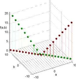
Figure 1. fp-S-theory forP1, where f(a, b) = fpd(Σa◦Sb).
Lemma 5.3. Retain the notation as in Example 5.2. When restrictingσ onto the categoryA, we have, for everym≥1,
(E5.3.1) fpdm(σn) =
(
1 n= 0,1,
0 otherwise.
Proof. When n = 0, (E5.3.1) is trivial. Let n = 1. For each set φ ∈ Φm,b, we
can assume thatφ={A(d1), A(d2,),· · ·, A(dm)}for a strictly increasing sequence {di|i= 1,2,· · ·, m}. For anyi < j, the (i, j)-entry of the adjacency matrix is
aij = dim(A(di), A(dj+ 1)) = 0.
ThusA(φ, σ) is a lower triangular matrix with
aii= dim(A(di), A(di+ 1)) = 1.
Henceρ(A(φ, σ)) = 1. So fpdm(σ) = 1.
Similarly, fpdm(σn) = 0 when n >1 as dim(A(di), A(di+ 2)) = 0 for alli.
Let n < 0. Let φ = {A(d1), A(d2,),· · ·, A(dm)} ∈ Φm,b where di are strictly
decreasing. Thenaij = dim(A(di), A(dj+n)) = 0 for alli≤j. Thusρ(A(φ, σn)) =
Example 5.4. Consider the quiver A2
(E5.4.1) •2←− •1.
LetPi (respectively,Ii) be the projective (respectively, injective) leftkA2-modules corresponding to verticesi, fori= 1,2, It is well-known that there are only three indecomposable left modules overA2, with Auslander-Reiten quiver (or AR-quiver, for short)
(E5.4.2) P2−→P1(=I2)−→I1
where each arrow represents a nonzero homomorphism (up to a scalar) [Sc1, Ex.1.13, pp.24-25]. The AR-translation (or translation, for short)τis determined byτ(I1) =
P2. Let T be Db(Mod
f.d.−kA2). The Auslander-Reiten theory can be extended
from the module category to the derived category. It is direct that, inT, we have the AR-quiver of all indecomposable objects
(E5.4.3)
❅ ❅
❘ ✒ ❅❅❘ ✒ ❅❅❘ ✒ ❅❅❘ ✒
P2[−1]
P1[−1]
I1[−1]
P2
P1=I2
I1
P2[1]
P1[1]
I1[1]
. . . .
The above represents all possible nonzero morphisms (up to a scalar) between non-isomorphic indecomposable objects in T. Note thatT has a Serre functor S
and that the AR-translationτcan be extended to a functor ofT such thatS= Σ◦τ
[RVdB, Proposition I.2.3] or [Cr, Remarks (2), p. 23]. After we identifying
P2[i]↔A(3i), P1[i]↔A(3i+ 1), I1[i]↔A(3i+ 2),
(E5.4.3) agrees with (E5.2.1). Using the above identification, at least when re-stricted to objects, we have
Σ(A(i))∼=A(i+ 3),
(E5.4.4)
τ(A(i))∼=A(i−2),
(E5.4.5)
S(A(i))∼=A(i+ 1).
(E5.4.6)
It follows from the definition of the AR-quiver [ARS, VII] that the degree ofτ is −2, see also [AS, Picture on p. 131]. Equation (E5.4.5) just means that the degree ofτ is−2.
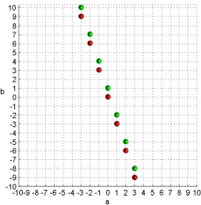
By equation (E5.4.6), the Serre functor S satisfies the property of σ defined in Example 5.2. By Lemma 5.3 or (E5.3.1), we have
fpdn(Σa◦Sb) = fpdn(σ3a+b) = (
1 3a+b= 0,1,
0 otherwise.
Therefore the fp-S-theory of T is given as above, and given as in Figure 2 (next page).
In particular, we have proven
fpgldim(Db(Mod
f.d.−kA2)) = fpd(Db(Modf.d.−kA2)) = fpd(Σ) = 0,
Figure 2. fp-S-theory forA2
5.3. An example of non-integral Frobenius-Perron dimension. In the next example, we “glue”K2 in (E5.1.3) andA2in (E5.4.1) together.
Example 5.5. LetG2be the quiver
(E5.5.1) •1
γ %
%
β
• 2
α
b
b
consisting of two vertices 1 and 2, with arrowα: 2→1 andβ, γ: 1→2 satisfying relations
(E5.5.2) R: βα=γα= 0, αβ=αγ = 0.
Note that (G2, R) is a quiver with relations. The corresponding quiver algebra with relations is a 5-dimensional algebra
A=ke1+ke2+kα+kβ+kγ
satisfying, in addition to (E5.5.2),
(E5.5.4) e2α= 0, αe1= 0, e1β=e1γ= 0, βe2=γe2= 0,
and
(E5.5.5) αe2=α=e1α, βe1=β =e2β, γe1=γ=e2γ.
We can use the following matrix form to represent the algebraA
A=
For eachi= 1,2, letSibe the left simpleA-module corresponding to the vertex
i and Pi be the projective cover of Si. ThenP1 ∼=Ae1 is isomorphic to the first column ofA, namely,
ke1
kβ+kγ
; andP2∼=Ae2is isomorphic to the second column
ofA, namely,
We will show that the Frobenius-Perron dimension of the category of finite di-mensional representations of (G2, R) is √2, by using several lemmas below that contain some detailed computations.
Lemma 5.6. Let V = (V1, V2) be a representation of(G2, R). LetW = imαand
K= kerα. Take ak-space decompositionV2=W⊕KwhereW ∼=W. Then there is a decomposition of(G2, R)-representationsV ∼= (W⊕T, W⊕K)∼= (W , W)⊕(T, K) where α is the identity when restricted to W (and identifying W with W)and is zero when restricted toK, whereβ and γare zero when restricted to W.
Proof. Since W = im α, V2 ∼= W ⊕K where K = kerα and W ∼= W. Write
V1 = W ⊕T for some k-subspace T ⊆ V1. The assertion follows by using the
relations in (E5.5.2).
Recall that A2 is the quiver given in (E5.4.1) and K2 is the Kronecker quiver given in (E5.1.3). By the above lemma, the subrepresentation (W, W) (where we identify W with W) is in fact a representation of
ke1 kα
0 ke2
(∼= kA2) and the
subrepresentation (T, K) is a representation of
Lemma 5.7. Supposek is of characteristic zero. The following is a complete list of indecomposable representations of (G2, R).
(5) S1,n= (T, K)withdimT =n+1anddimK=n, whereα= 0,β= (In,0)τ
and γ= (0, In)τ.
As a consequence,kG2/(R)is of tame representation type[Definition 7.1]. Proof. (1) By Lemma 5.6, this is the only case that could happen when α 6= 0. Now we assumeα= 0.
(2,3,4,5) Ifα= 0, then we are working with representations of Kronecker quiver
K2 (E5.1.3). The classification follows from a classical result of Kronecker [Ben, Theorem 4.3.2].
By (1-5), for each integern, there are only finitely many 1-parameter families of indecomposable representations of dimensionn. Therefore A is of tame
represen-tation type.
The following is a consequence of Lemma 5.7 and a direct computation.
Lemma 5.8. Retain the hypotheses of Lemma 5.7. The following is a complete list of brick representations of (G2, R).
(1) P2∼= (k,k), where α=I1 andβ=γ= 0.
(2) X1(λ) = (k,k), whereα= 0,β=I1 andγ=λI1 for someλ∈k. (3) Y1= (k,k), whereα= 0,β= 0 andγ=I1.
(4) S2,n for n≥0. (5) S1,n for n≥0.
The set Φ1,b consists of the above objects.
LetX1(∞) denoteY1. We have the following short exact sequences of (G2, R )-representations
0→S1→P2→S2→0,
0→S2→X1(λ)→S1→0,
0→S2n+1→S2,n→S1n→0,
0→S2n→S1,n→S1n+1→0,
0→S22→S2,n→S1,n−1→0,
where n ≥ 1 for the last exact sequence, and have the following nonzero homs, whereA=kG2/(R),
HomA(X1(λ), S1,n)6= 0, ∀n≥1
HomA(S2,n, X1(λ))6= 0, ∀n≥1
HomA(S2,m, S2,n)6= 0, ∀m≤n
HomA(S1,n, S1,m)6= 0, ∀m≤n
HomA(S2,n, S1,m)6= 0, ∀m+n≥1
Lemma 5.9. Retain the hypotheses of Lemma 5.7. The following is the complete list of zero hom-sets between brick representations of G2 in both directions.
(1) HomA(X1(λ), X1(λ′)) = HomA(X1(λ′), X1(λ)) = 0 ifλ6=λ′ ink∪ {∞}.
(2) HomA(S1, S2) = HomA(S2, S1) = 0.
As a consequence, if φ ∈ Φn,b for some n ≥ 2, then φ = {S1, S2} or φ =
{X1(λi)}n
i=1 for different parameters {λ1,· · ·, λn}.
We also need to compute the Ext1A-groups.
(1) Ext1A(X1(λ), X1(λ)) = HomA(X1(λ), X1(λ)) =k.
Remark 5.11. In fact, one can show the following stronger version of Lemma 5.10(5,6).
(5’) Ext1A(S2,n, S2,n) = 0 for alln.
(6’) Ext1A(S1,n, S1,n) = 0 for alln.
Proof of Lemma 5.10. (1,2) Consider a minimal projective resolution ofX1(λ)
P1→P2 fλ
Applying HomA(−, X1(λ′)) to the truncated projective resolution of the above, we
obtain the following complex
k←−−−−0 k←−−−−g k←−0.
Ifg is zero, this is case (1). Ifg6= 0, this is case (2).
(3) The proof is similar to the above by considering minimal projective resolu-tions ofS1and S2.
(4) This is clear sinceP2 is a projective module.
(5,6) Let S be either S2,n or S1,n. By Example 5.1, fpd(Modf.d−kK2) = 1.
This implies that
dim Ext1kK2(S, S)≤1 whereS is considered as an indecomposableK2-module.
Let us make a comment before we continue the proof. Following a more careful analysis, one can actually show that
Ext1kK2(S, S) = 0.
Using this fact, the rest of the proof would show the assertions (5’,6’) in Remark 5.11.
Now we continue the proof. There is a projective coverPb 1
f
−→S so that kerf is a direct sum of finitely many copies of S2. Since P2 is the projective cover of S2, we have a minimal projective resolution
−→Pa
2 −→P1b −→S−→0
for somea, b. In the category Modf.d−kK2, we have a minimal projective resolution
ofS
whereS2 is a projectivekK2-module. Hence we have a morphism of complexes dimension at most 1. Sinceg is an isomorphism, the cokernel ofhhas dimension at most 1. This implies that Ext1A(S, S) has dimension at most 1.
Proposition 5.12. Let Abe the categoryModf.d.−A whereA is in Example 5.5.
(1) fpdnA=
Proof. (1) This is a consequence of Lemmas 5.9 and 5.10. Parts (2,3) follow from
part (1).
Remark 5.13. Let A be the algebra given in Example 5.5. We list some facts, comments and questions.
(1) The algebraAis non-connectedN-graded Koszul. (2) The minimal projective resolutions ofS1andS2are
· · · −→P⊕4
non-integral (or irrational) fpd. It is unknown if there is a finite dimensional algebraAsuch that fpd(Modf.d.−A) is transcendental.
(5) Several authors have studied the connection between tame-wildness and complexity [BS, ES, Fa, FW, Kul, Ri]. The algebraAis probably the first explicit example of a tame algebra with infinite complexity.
(6) It follows from part (3) that the fp-curvature ofA:=Db(Mod
f.d.−A) is
√ 2 (some details are omitted). As a consequence, fpg(A) =∞. By Theorem 8.3, the complexity ofA is∞. We don’t know what fpdAis.
6. σ-decompositions
We fix a categoryC and an endofunctor σ. For a set of bricksB in C (or a set of atomic objects whenC is triangulated), we define
fpdn |B(σ) = sup{ρ(A(φ, σ)) | φ:={X1,· · ·, Xn} ∈Φn,b, and Xi ∈B ∀i}.
Lemma 6.1. Let n be a positive integer. Suppose that B has a σ-decomposition {Bλ}
φin the order that suggested by (E6.1.1), then the adjacency matrix of (φ, σ) is of the form
wheresi is the size ofAii, which is no more thann. Therefore
ρ(A(φ, σ)) = max
i {ρ(Aii)} ≤λ∈Λ,msup≤n{fpd m
|Bλ(σ)}.
The assertion follows.
We give some examples ofσ-decompositions.
Example 6.2. LetAbe an abelian category andAbe the derived categoryDb(A).
(1) Suppose that αis an endofunctor of A and α is the induced endofunctor
of A. For each n ∈ Z, let Bn := {M[−n] | M is a brick in A} and B :=Sn∈ZBn. IfMi[−ni]∈Bni, fori= 1,2, such thatn1< n2, then
HomA(M1[−n1], α(M2[−n2])) = ExtnA1−n2(M1, α(M2)) = 0.
ThenB has aα-decomposition{Bn}
n∈Z based onZ.
(2) Supposeg := gldimA<∞. Letσ be the functor Σg◦α. For eachn∈Z, letBn :={M[n]|M is a brick inA} andB :=S
n∈ZBn. IfMi[ni]∈Bni,
fori= 1,2, such thatn1< n2, then
HomA(M1[n1], σ(M2[n2])) = ExtAn2−n1+g(M1, α(M2)) = 0.
ThenB has aσ-decomposition{Bn}
n∈Zbased on Z.
Example 6.3. LetC be a smooth projective curve and letAbe the the category
of coherent sheaves overC. Every coherent sheaf overCis a direct sum of a torsion subsheaf and a locally free subsheaf. Define
B0={T is a torsion brick object in A}, B−1={F is a locally free brick object in A}
and
B=B−1∪B0.
Letσbe the functorE1:= Ext1
A(−,−). IfF ∈B−1 andT ∈B0, then
Ext1A(F, T) = 0.
Hence,B has anE1-decomposition based on the totally ordered set Λ :={−1,0}.
The next example is given in [BB].
Example 6.4. LetC be an elliptic curve. Let Abe the the category of coherent
sheaves overC andAbe the derived categoryDb(A).
First we consider coherent sheaves. Let Λ be the totally ordered setQ∪ {+∞}. The slope of a coherent sheafX 6= 0 [BB, Definition 4.6] is defined to be
µ(X) := χ(X) rk(X) ∈Λ
whereχ(X) is the Euler characteristic ofXand rk(X) is the rank ofX. IfX andY
are bricks such thatµ(X)< µ(Y), by [BB, Corollary 4.11],X andY are semistable, and thus by [BB, Proposition 4.9(1)], HomA(Y, X) = 0. By Serre duality (namely,
Calabi-Yau property),
(E6.4.1) HomA(X, Y[1]) = Ext1A(X, Y) = HomA(Y, X)∗= 0.
Write B = Φ1,b(A) andBλ be the set of (semistable) bricks with slope λ. Then B = Sλ∈ΛBλ. By (E6.4.1), Ext1
A(X, Y) = 0 when X ∈ Bλ and Y ∈ Bν with
λ < ν. HenceB has an E1-decomposition. By Lemma 6.1, for everyn≥1,
fpdn(E1) = fpdn|B(E1)≤ sup λ∈Λ,m≤n{
fpdm|Bλ(E1)}.
Next we compute fpdn|Bλ(E1). Let SSλ be the full subcategory of A
con-sisting of semistable coherent sheaves of slope λ. By [BB, Summary], SSλ is an
abelian category that is equivalent toSS∞. Therefore one only needs to compute fpdn|B∞(E1) in the categorySS∞. Note thatSS∞ is the abelian category of
tor-sion sheaves and every brick object in SS∞ is of the form O
In this case, A(φ, E1) is the identity matrix. Consequently, ρ(A(φ, E1)) = 1.
This shows that fpdn|Bλ(E1) = fpdn|B∞(E1) = 1 for all n ≥ 1. It is clear
that fpdn(E1)≥fpdn
|B∞(E1) = 1. Combining with Lemma 6.1, we obtain that
fpdn(E1) = 1 for alln. (The above approach works for functors other thanE1.)
Finally we consider the fp-dimension for the derived categoryA. It follows from Theorem 3.5(3) that
fpdn(Σ) = fpdn(E1) = 1 for alln≥1. By definition,
fpd(A) = fpd(A) = 1.
As we explained before fpd is an indicator of the representation types of cate-gories.
Drozd-Greuel studied a tame-wild dichotomy for vector bundles on projective curves [DrG] and introduced the notion of VB-finite, VB-tame and VB-wild sim-ilar to the corresponding notion in the representation theory of finite dimensional algebras. In [DrG] Drozd-Greuel showed the following:
LetCbe a connected smooth projective curve. Then (a) C is VB-finite if and only if CisP1.
(b) C is VB-tame if and only if Cis elliptic (that is, of genus 1). (c) C is VB-wild if and only if Chas genusg≥2.
We now prove a fp-version of Drozd-Greuel’s result [DrG, Theorem 1.6]. We thank Max Lieblich for providing ideas in the proof of Proposition 6.5(3) next.
Proposition 6.5. Suppose k=C. Let Xbe a connected smooth projective curve and letg be the genus ofX.
(1) If g= 0 orX=P1, then fpd Db(coh(X)) = 1.
(2) If g= 1 orXis an elliptic curve, then fpd Db(coh(X)) = 1.
(3) If g≥2, thenfpd Db(coh(X)) =∞.
Proof. (1) The assertion follows from (E5.1.4). (2) The assertion follows from Example 6.4.
(3) By Theorem 3.5(4), fpd(Db(coh(X))) = fpd(coh(X)). Hence it suffices to
show that fpd(coh(X)) =∞. For eachn, let{xi}n
i=1be a set ofndistinct points onX. By [DrG, Lemma 1.7],
we might further assume that 2xi6∼xj+xk for all i6=j, as divisors onX. Write Ei := O(xi) for all i. By [DrG, p.11], HomOX(Ei,Ej) = 0 for all i 6=j, which is
also a consequence of a more general result [HL, Proposition 1.2.7]. It is clear that HomOX(Ei,Ei) =kfor alli. Letφnbe the set{E1, . . . ,En}. Then it is a brick set of
non-isomorphic vector bundles onX(which are stable with rank(Ei) = deg(Ei) = 1
for alli).
Define the sheaf Hij = Hom(Ei,Ej) for all i, j. Then deg(Hij) = 0. By the
Riemann-Roch Theorem, we have
0 = deg(Hij)
=χ(Hij)−rank(Hij)χ(OX)
= dim HomOX(Ei,Ej)−dim Ext 1
OX(Ei,Ej)−(1−g)