Geometry
Our tour of theoretical physics begins with geometry, and there are two reasons for this. One is that the framework of space and time provides, as it were, the stage upon which physical events are played out, and it will be helpful to gain a clear idea of what this stage looks like before introducing the cast. As a matter of fact, the geometry of space and time itself plays an active role in those physical processes that involve gravitation (and perhaps, according to some speculative theories, in other processes as well). Thus, our study of geometry will culminate, in chapter 4, in the account of gravity offered by Einstein’s general theory of relativity. The other reason for beginning with geometry is that the mathematical notions we develop will reappear in later contexts.
To a large extent, the special and general theories of relativity are ‘negative’ theories. By this I mean that they consist more in relaxing incorrect, though plausible, assumptions that we are inclined to make about the nature of space and time than in introducing new ones. I propose to explain how this works in the following way. We shall start by introducing a prototype version of space and time, called a ‘differentiable manifold’, which possesses a bare minimum of geometrical properties—for example, the notion of length is not yet meaningful. (Actually, it may be necessary to abandon even these minimal properties if, for example, we want a geometry that is fully compatible with quantum theory and I shall touch briefly on this in chapter 15.) In order to arrive at a structure that more closely resembles space and time as we know them, we then have to endow the manifold with additional properties, known as an ‘affine connection’ and a ‘metric’. Two points then emerge: first, the common-sense notions of Euclidean geometry correspond to very special choices for these affine and metric properties; second, other possible choices lead to geometrical states of affairs that have a natural interpretation in terms of gravitational effects. Stretching the point slightly, it may be said that, merely byavoidingunnecessary assumptions, we are able to see gravitation as something entirely to be expected, rather than as a phenomenon in need of explanation.
To me, this insight into the ways of nature is immensely satisfying, and it
is in the hope of communicating this satisfaction to readers that I have chosen to approach the subject in this way. Unfortunately, the assumptions we are to avoid are, by and large,simplifyingassumptions, so by avoiding them we let ourselves in for some degree of complication in the mathematical formalism. Therefore, to help readers preserve a sense of direction, I will, as promised in chapter 1, provide an introductory section outlining a more traditional approach to relativity and gravitation, in which we ask how our na¨ıve geometrical ideas must be modified to embrace certain observed phenomena.
2.0
The Special and General Theories of Relativity
2.0.1 The special theory
The special theory of relativity is concerned in part with the relation between observations of some set of physical events in two inertial frames of reference that are in relative motion. By an inertial frame, we mean one in which Newton’s first law of motion holds:
Every body continues in its state of rest, or of uniform motion in a right line, unless it is compelled to change that state by forces impressed on it.
(Newton 1686)
It is worth noting that this definition by itself is in danger of being a mere tautology, since a ‘force’ is in effect defined by Newton’s second law in terms of the acceleration it produces:
The change of motion is proportional to the motive force impressed; and is made in the direction of the right line in which that force is impressed. (Newton 1686)
So, from these definitions alone, we have no way of deciding whether some observed acceleration of a body relative to a given frame should be attributed, on the one hand, to the action of a force or, on the other hand, to an acceleration of the frame of reference. Eddington has made this point by a facetious re-rendering of the first law:
Every body tends to move in the track in which it actually does move, except insofar as it is compelled by material impacts to follow some other track than that in which it would otherwise move.
(Eddington 1929)
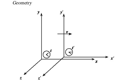
Figure 2.1.Two systems of Cartesian coordinates in relative motion.
that cannot be eliminated. To proceed, we must take it as established that, in principle, frames of reference can be constructed, relative to which any isolated body will, as a matter of fact, always refuse to accelerate. These frames we call inertial.
Obviously, any two inertial frames must either be relatively at rest or have a uniform relative velocity. Consider, then, two inertial frames,SandS′(standing forSystems of coordinates) with Cartesian axes so arranged that thexandx′axes lie in the same line, and suppose thatS′ moves in the positivex direction with speedv relative to S. Taking y′ parallel to y andz′ parallel toz, we have the arrangement shown in figure 2.1. We assume that the sets of apparatus used to measure distances and times in the two systems are identical and, for simplicity, that both clocks are adjusted to read zero at the moment the two origins coincide. Suppose that an event at the coordinates(x,y,z,t)relative toS is observed at(x′,y′,z′,t′)relative toS′. According to the Galilean, or common-sense, view of space and time, these two sets of coordinates must be related by
x′=x−vt y′=y z′=z t′=t. (2.1)
Since the path of a moving particle is just a sequence of events, we easily find that its velocity relative to S, in vector notationu = dx/dt, is related to its velocity u′ = dx′/dt′ relative to S′ by u′ = u−v, with v = (v,0,0), and that its acceleration is the same in both frames,a′=a.
called the speed of light. Indeed, the speed of light is predicted by Maxwell’s electromagnetic theory to be(ǫ0µ0)−1/2(inSIunits, whereǫ0andµ0are called
the permittivity and permeability of free space, respectively) but the theory does not single out any special frame relative to which this speed should be measured. For quite some time after the appearance of Maxwell’s theory (published in its final form in 1864; see also Maxwell (1873)), it was thought that electromagnetic radiation consisted of vibrations of a medium, the ‘luminiferous ether’, and would travel at the speedcrelative to the rest frame of the ether. However, a number of experiments cast doubt on this interpretation. The most celebrated, that of Michelson and Morley (1887), showed that the speed of the Earth relative to the ether must, at any time of year, be considerably smaller than that of its orbit round the Sun. Had the ether theory been correct, of course, the speed of the Earth relative to the ether should have changed by twice its orbital speed over a period of six months. The experiment seemed to imply, then, that light always travels at the same speed,c, relative to the apparatus used to observe it.
In his paper of 1905, Einstein makes the fundamental assumption (though he expresses things a little differently) thatlight travels with exactly the same speed, c, relative to any inertial frame. Since this is clearly incompatible with the Galilean transformation law given in (2.1), he takes the remarkable step of modifying this law to read
x′= x−vt
(1−v2/c2)1/2 y
′=y
z′=z t′= t−vx/c
2
(1−v2/c2)1/2.
(2.2)
These equations are known as the Lorentz transformation, because a set of equations having essentially this form had been written down by H A Lorentz (1904) in the course of his attempt to explain the results of Michelson and Morley. However, Lorentz believed that his equations described a mechanical effect of the ether upon bodies moving through it, which he attributed to a modification of intermolecular forces. He does not appear to have interpreted them as Einstein did, namely as a general law relating coordinate systems in relative motion. The assumptions that lead to this transformation law are set out in exercise 2.1, where readers are invited to complete its derivation. Here, let us note that (2.2) does indeed embody the assumption that light travels with speed c relative to any inertial frame. For example, if a pulse of light is emitted from the common origin ofS andS′ att =t′ =0, then the equation of the resulting spherical wavefront at timetrelative toSisx2+y2+z2=c2t2. Using the transformation (2.2), we easily find that its equation at timet′relative toS′isx′2+y′2+z′2=c2t′2.
these equations require us to make in our view of space and time. On the face of it, equations (2.1) or (2.2) simply tell us how to relate observations made in two different frames of reference. At a deeper level, however, they contain information about the structure of space and time that is independent of any frame of reference. Consider two events with spacetime coordinates(x1,t1)and(x2,t2)relative to
S. According to the Galilean transformation, the time intervalt2−t1between
them relative to S is equal to the intervalt2′ −t1′ relative to S′. In particular, it may happen that these two events are simultaneous, so thatt2−t1 = 0, and
this statement would be equally valid from the point of view of either frame of reference. For two simultaneous events, the spatial distances between them, |x1−x2|and|x′
1−x2′|are also equal. Thus, the time interval between two events
and the spatial distance between two simultaneous events have the same value in everyinertial frame, and hence have real physical meanings that are independent of any system of coordinates. According to the Lorentz transformation (2.2), however, both the time interval and the distance have different values relative to different inertial frames. Since these frames are arbitrarily chosen by us, neither the time interval nor the distance has any definite, independent meaning. The one quantity that does have a definite, frame-independent meaning is theproper time intervalτ, defined by
c2τ2=c2t2−x2 (2.3)
wheret =t2−t1andx = |x2−x1|. By using (2.2), it is easy to verify that
c2t′2−x′2is also equal toc2τ2.
We see, therefore, that the Galilean transformation can be correct only in a Galilean spacetime; that is, a spacetime in which both time intervals and spatial distances have well-defined meanings. For the Lorentz transformation to be correct, the structure of space and time must be such that only proper-time intervals are well defined. There are, as we shall see, many such structures. The one in which the Lorentz transformation is valid is calledMinkowski spacetime after Hermann Minkowski who first clearly described its geometrical properties (Minkowski, 1908). These properties are summarized by the definition (2.3) of proper time intervals. In this definition, the constantcdoes not refer to the speed of anything. Although it has the dimensions of velocity, its role is really no more than that of a conversion factor between units of length and time. Thus, although the special theory of relativity arose from attempts to understand the propagation of light, it has nothing to do with electromagnetic radiation as such. Indeed, it is not in essence about relativity either! Its essential feature is the structure of space and time expressed by (2.3), and the law for transforming between frames in relative motion serves only as a clue to what this structure is. With this in mind, Minkowski (1908) says of the name ‘relativity’ that it ‘. . . seems to me very feeble’.
The laws by which the states of physical systems undergo change are not affected, whether these changes of state be referred to the one or the other of two systems of coordinates in uniform translatory motion.
(Einstein 1905)
Any inertial frame, that is to say, should be as good as any other as far as the laws of physics are concerned. Mathematically, this means that the equations expressing these laws should becovariant—they should have the same form in any inertial frame. Consider, for example, two objects, with massesm1andm2,
situated atx1andx2on thexaxis ofS. According to Newtonian mechanics and
the Newtonian theory of gravity, the equation of motion for particle 1 is
m1
d2x1
dt2 =(Gm1m2)
x2−x1
|x2−x1|3
(2.4)
where G ≃ 6.67× 10⁻¹¹N m2kg−2 is Newton’s gravitational constant. If spacetime is Galilean and the transformation law (2.1) is valid, then d2x′/dt′2= d2x/dt2and(x′2−x1′) =(x2−x1), so in S′ the equation has exactly the same
form and Einstein’s principle is satisfied. In Minkowski spacetime, we must use the Lorentz transformation. The acceleration relative to S is not equal to the acceleration relative to S′ (see exercise 2.2), but worse is to come! On the right-hand side,x1 andx2refer to two events, namely the objects reaching
these two positions, which occur simultaneously as viewed fromS. As viewed fromS′, however, these two events are separated by a time interval(t′
2−t1′)=
(x1′ −x2′)v/c2, as readers may easily verify from (2.2). In Minkowski spacetime, therefore, (2.4) does not respect the principle of relativity. It is unsatisfactory as a law of motion because it implies that there is a preferred inertial frame, namely S, relative to which the force depends only on the instantaneous separation of the two objects; relative to any other frame, it depends on the distance between their positions at different times, and also on the velocity of the frame of reference relative to the preferred one. Actually, we do not knowa priorithat there is no such preferred frame. In the end, we trust the principle of relativity because the theories that stem from it explain a number of observed phenomena for which Newtonian mechanics cannot account.
We might imagine that electrical forces would present a similar problem, since we obtain Coulomb’s law for particles with charges q1 and q2 merely
by replacing the constant in parentheses in (2.4) with −q1q2/4π ǫ0. In fact,
a frame in which the particle is moving, we also see a magnetic field. Moreover, disturbances in these fields are transmitted at the speed of light. The problem of simultaneity is avoided because a second particle responds not directly to the first one, but rather to the electromagnetic field at its own position. The expression analogous to the right-hand side of (2.4) for the Coulomb force is valid only when there is a frame of reference in which particle 2 can be considered fixed, and then only as an approximation.
2.0.2 The general theory
The experimental fact that eventually led to the special theory was, as we have seen, the constancy of the speed of light. The general theory, and the account that it provides of gravitation, also spring from a crucial fact of observation, namely the equality of inertial and gravitational masses. In (2.4), the massm1appears in
two different guises. On the left-hand side,m1denotes theinertial mass, which
governs the response of the body to a given force. On the right-hand side, it denotes thegravitational mass, which determines the strength of the gravitational force. The gravitational mass is analogous to the electric charge in Coulomb’s law and, since the electrical charge on a body is not necessarily proportional to its mass, there is no obvious reason why the gravitational ‘charge’ should be determined by the mass either. The equality of gravitational and inertial masses is, of course, responsible for the fact that the acceleration of a body in the Earth’s gravitational field is independent of its mass, and this has been familiar since the time of Galileo and Newton. It was checked in 1889 to an accuracy of about one part in 109by E¨otv¨os, whose method has been further refined more recently by R H Dicke and his collaborators.
It seemed to Einstein that this precise equality demanded some explanation, and he was struck by the fact thatinertial forcessuch as centrifugal and Coriolis forces are proportional to the inertial mass of the body on which they act. These inertial forces are often regarded as ‘fictitious’, in the sense that they arise from the use of accelerating (and therefore non-inertial) frames of reference. Consider, for example, a spaceship far from any gravitating bodies such as stars or planets. When its motors are turned off, a frame of referenceSfixed in the ship is inertial provided, as we assume, that it is not spinning relative to distant stars. Relative to this frame, the equation of motion of an object on which no forces act is md2x/dt2 = 0. Suppose the motors are started at timet = 0, giving the ship a constant accelerationain thexdirection.Sis now not an inertial frame. IfS′is the inertial frame that coincided withSfort <0, then the equation of the object is stillmd2x′/dt′2=0, at least until the object collides with the cabin walls. Using
Galilean relativity for simplicity, we havex′=x+12at2andt′=t, so relative to Sthe equation of motion is
md
2x
dt2 = −ma. (2.5)
and is definitely proportional to theinertialmass.
Einstein’s idea is that gravitational forces are of essentially the same kind as that appearing in (2.5), which means that the inertial and gravitational masses are necessarily identical. Suppose that the object in question is in fact a physicist, whose ship-board laboratory is completely soundproof and windowless. His sensation of weight, as expressed by (2.5), is equally consistent with the ship’s being accelerated by its motors or with its having landed on a planet at whose surface the acceleration due to gravity isa. Conversely, when he was apparently weightless, he would be unable to tell whether his ship was actually in deep space or freely falling towards a nearby planet. This illustrates Einstein’sprinciple of equivalence, according to which the effects of a gravitational field can locally be eliminated by using a freely-falling frame of reference. This frame is inertial and, relative to it, the laws of physics take the same form that they would have relative to any inertial frame in a region far removed from any gravitating bodies.
The word ‘locally’ indicates that the freely-falling inertial frame can usually extend only over a small region. Let us suppose that our spaceship is indeed falling freely towards a nearby planet. (Readers may rest assured that the pilot, unlike the physicist, is aware of this and will eventually act to avert the impending disaster.) If he has sufficiently accurate apparatus, the physicist can detect the presence of the planet in the following way. Knowing the standard landing procedure, he allows two small objects to float freely on either side of his laboratory, so that the line joining them is perpendicular to the direction in which he knows that the planet, if any, will lie. Each of these objects falls towards the centre of the planet, and therefore their paths slowly converge. As observed in the freely-falling laboratory, they do not accelerate in the direction of the planet, but they do accelerate towards each other, even though their mutual gravitational attraction is negligible. (The tendency of the cabin walls to converge in the same manner is, of course, counteracted by interatomic forces within them.) Strictly, then, the effects of gravity are eliminated in the freely-falling laboratory only to the extent that two straight lines passing through it, which meet at the centre of the planet, can be considered parallel. If the laboratory is small compared with its distance from the centre of the planet, then this will be true to a very good approximation, but the equivalence principle applies exactly only to an infinitesimal region.
of Galilean or Minkowski spacetime and interpret our observations accordingly. Consider again the expression for proper time intervals given in (2.3). It is valid when(x,y,z,t)refer to Cartesian coordinates in an inertial frame of reference. In the neighbourhood of a gravitating body, a freely-falling inertial frame can be defined only in a small region, so we write it as
c2(dτ )2=c2(dt)2−(dx)2 (2.6)
where dt and dx are infinitesimal coordinate differences. Now let us make a transformation to an arbitrary system of coordinates(x0,x1,x2,x3), each new coordinate being expressible as some function ofx,y,zandt. Using the chain rule, we find that (2.6) becomes
where the functions gµν(x)are given in terms of the transformation functions. They are components of what is called themetric tensor. In the usual version of general relativity, it is the metric tensor that embodies all the geometrical structure of space and time. Suppose we are given a set of functionsgµν(x)which describe this structure in terms of some system of coordinates{xµ}. According to the principle of equivalence, it is possible at any point (say X, with coordinates Xµ) to construct a freely falling inertial frame, valid in a small neighbourhood surroundingX, relative to which there are no gravitational effects and all other processes occur as in special relativity. This means that it is possible to find a set of coordinates(ct,x,y,z)such that the proper time interval (2.7) reverts to the form of (2.6). Using a matrix representation of the metric tensor, we can write
gµν(X)=ηµν ≡
whereηµνis the special metric tensor corresponding to (2.6).
This concludes our introductory survey of the theories of relativity. We have concentrated on the ways in which our common-sense ideas of spacetime geometry must be modified in order to accommodate two key experimental observations: the constancy of the speed of light and the equality of gravitational and inertial masses. It is clear that the modified geometry leads to modifications in the laws that govern the behaviour of physical systems, but we have not discussed these laws in concrete terms. That we shall be better equipped to do after we have developed some mathematical tools in the remainder of this chapter. At that stage, we shall be able to see much more explicitly how gravity arises from geometry.
2.1
Spacetime as a Differentiable Manifold
Our aim is to construct a mathematical model of space and time that involves as few assumptions as possible, and to be explicitly aware of the assumptions we do make. In particular, we have seen that the theories of relativity call into question the meanings we attach to distances and time intervals, and we need to be clear about these. The mathematical structure that has proved to be a suitable starting point, at least for a non-quantum-mechanical model of space and time, is called a differentiable manifold. It is a collection of points, each of which will eventually correspond to a unique position in space and time, and the whole collection comprises the entire history of our model universe. It has two key features that represent familiar facts about our experience of space and time. The first is that any point can be uniquely specified by a set of four real numbers, so spacetime is four-dimensional. For the moment, the exact number of dimensions is not important. Later on, indeed, we shall encounter some recent theories which suggest that there may be more than four, the extra ones being invisible to us. Even in more conventional theories, we shall find that it is helpful to consider other numbers of dimensions as a purely mathematical device. The second feature is a kind of ‘smoothness’, meaning roughly that, given any two distinct points, there are more points in between them. This feature allows us to describe physical quantities such as particle trajectories or electromagnetic fields in terms of differentiable functions and hence to do theoretical physics of the usual kind. We do not know for certain that space and time are quite as smooth as this, but at least there is no evidence for any granularity down to the shortest distances we are able to probe experimentally.
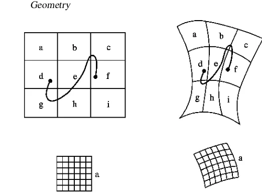
Figure 2.2. A deformable sheet of rubber, divided into several regions. Although there is no definite distance between the points indicated by
•
, there are always other points between them, because any curve joining them must pass through at least one of the regions b, e and h.on the sheet, because it can be deformed at will. No matter how it is deformed, however, any given region is still surrounded by the same neighbouring regions. Given a point in d and another in f, we can never draw a line between them that does not pass through at least one of regions b, e and h. The same holds, moreover, of more finely subdivided regions, as shown for subdivisions of a, each of which could be further subdivided, and so on. In this sense, points on the sheet are smoothly connected together. The smoothness would be lost if the rubber were vaporized, the individual molecules being considered as the collection of points. Mathematically, the kind of smoothness we want is a property of the real line (that is, the set of all real numbers, denoted byR). So, as part of the definition of the manifold, we demand that it should be possible to set up correspondences (called ‘maps’) between points of the manifold and sets of real numbers. We shall next look at the topological properties of real numbers, and then see how we can ensure that the manifold shares them.
2.1.1 Topology of the real lineRand ofR
d
The topological properties we are interested in are expressed in terms of ‘open sets’, which are defined in the following way. Anopen interval(a,b)is the set of all points (real numbers)xsuch thata <x<b:
· · · ( | ) · · ·
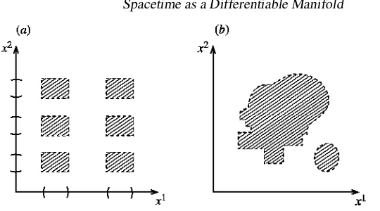
Figure 2.3.(a) An open set inR
2. It is a union of open rectangles constructed from unions
of open intervals in the two copies ofRwhich form thex
1andx2axes. (b) Another open
set inR
2, which can be constructed as a union of open rectangles.
The end pointsx = a andx = b are excluded. Consequently,anypointx in
(a,b)can be surrounded by another open interval(x−ǫ,x+ǫ), all of whose points are also in(a,b). For example, however closexis toa, it cannot be equal toa. There are always points betweenaandx, and ifx is closer toathan tob, we can takeǫ=(x−a)/2. Anopen setofRis defined as any union of 1, 2, 3,
. . .open intervals:
( ) or ( ) ( ) or ( ) ( ) ( )
etc. (Theunion A∪B∪C· · ·of a number of sets is defined as the set of all points that belong to at least one ofA,B,C, . . .. Theintersection A∩B∩C· · ·is the set of all points that belong to all the setsA,B,C, . . ..) In addition, the empty set, which contains no points, is defined to be an open set.
The spaceR
2 is the set of all pairs of real numbers(x1,x2), which can be
envisaged as an infinite plane. The definition of open sets is easily extended toR
2,
as illustrated in figure 2.3. Ifx1lies in a chosen open interval on the horizontal axis, andx2in a chosen open interval on the vertical axis, then(x1,x2)lies in an open rectangle corresponding to these two intervals. Any union of open rectangles is an open set. Since the rectangles can be arbitrarily small, we can say that any region bounded by a closed curve, but excluding points actually on the curve, is also an open set, and so is any union of such regions. Obviously, the same ideas can be further extended toR
d, which is the set of alld-tuples of real numbers
(x1,x2, . . . ,xd).
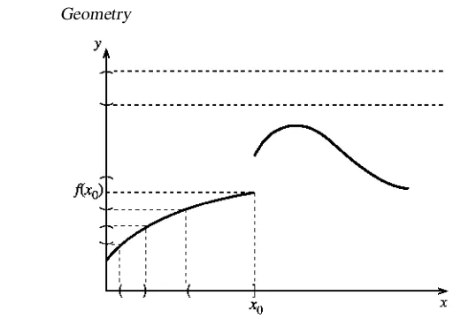
Figure 2.4. The graphy = f(x)of a function which is discontinuous atx0. Any open
interval ofywhich includes f(x0)has an inverse image on thexaxis which is not open.
The inverse image of an interval inywhich contains no values of f(x)is the empty set.
inverse image of any open set on the y axis is an open set on the x axis. The example shown fails to be continuous because the inverse image of any open interval containing f(x0)contains an interval of the type(x1,x0], which includes
the end pointx0and is therefore not open. (Readers who are not at home with this
style of argument should spend a short while considering the implications of these definitions: why, for example, is it necessary to include not only open intervals but also their unions and the empty set as open sets?)
The open sets ofR
d have two fairly obvious properties: (i) any union of
open sets is itself an open set; (ii) any intersection of a finite number of open sets is itself an open set. Given any space (by which we mean a set of points), suppose that a collection of subsets of its points is specified, such that any union or finite intersection of them also belongs to the collection. We also specify that the entire space (which counts as a subset of itself) and the empty set belong to the collection. Then the subsets in this collection may, by analogy, be calledopen sets. The collection of open sets is called atopologyand the space, together with its topology, is called atopological space. It is, of course, possible to endow a given space with many different topologies. For example, the collection of all subsets of the space clearly satisfies all the above conditions, and is called the discrete topology. By endowing the real line with this topology, we would obtain a new definition of continuity—it would not be a particularly useful definition, however, as any function at all would turn out to be continuous. The particular topology ofR
d described above is called thenatural topologyand is the one we
shall always use.
It is important to realize that a topology is quite independent of any notion of distance. For instance, a sheet of paper may be regarded as a part of R
The natural topology reflects the way in which its points fit together to form a coherent structure. If it is used to draw figures in Euclidean geometry, then the distance D between two points is defined by the Pythagoras rule as D = (x)2+(y)21/2. But it might equally well be used to plot the mean atmospheric concentration of carbon monoxide in central London (represented byy) as a function of time (represented byx), in which case Dwould have no sensible meaning.
A topology imposes two kinds of structure on the space. The local topology—the way in which open sets fit inside one another over small regions— determines the way in which notions like continuity apply to the space. Theglobal topology—the way in which the open sets can be made to cover the whole space— determines its overall structure. Thus, the plane, sphere and torus have the same local structure but different global structures. Physically, we have no definite information about the global topology of spacetime, but its local structure seems to be very similar to that ofR
4 (though we shall encounter speculative theories
that call this apparently simple observation into question).
2.1.2 Differentiable spacetime manifold
In order that our model of space and time should be able to support continuous and differentiable functions of the sort that we rely on to do physics, we want it (for now) to have the same local topology asR
4. First of all, then, it must be
a topological space. That is, it must have a collection of open sets, in terms of which continuous functions can be defined. Second, the structure of these open sets must be similar, within small regions, to the natural topology ofR
4. To this
end, we demand that every point of the space belong to at least one open set, all of whose points can be put into a one-to one correspondence with the points of some open set ofR
4. More technically, the correspondence is a one-to-one
mapping of the open set of the spaceontothe open set of R
4, which is to say
that every point of the open set in the space has a unique image point in the open set ofR
4 andvice versa. We further demand that this mapping be continuous,
according to our previous definition. When these conditions are met, the space is called amanifold. The existence of continuous mappings between the manifold andR
4 implies that a function f defined on the manifold (that is, one that has a
value f(P)for each pointPof the manifold) can be re-expressed as a functiong defined onR
4, so that f(P)=g(x0, . . . ,x3), where(x0, . . . ,x3)is the point of
R
4corresponding toP. In this way, continuous functions defined on the manifold
inherit the characteristics of those defined onR
4.
Figure 2.5.A coordinate patch on a two-dimensional manifold. Each point in the patch is mapped to a unique image point in a region ofR
2andvice versa.
Figure 2.6. Two overlapping coordinate patches. A point in the overlap region can be identified using either set of coordinates.
manifold for each set of coordinate values—so there are no points ‘missing’ from the manifold, and also that there are no ‘extra’ points that cannot be assigned coordinates. Within a coordinate patch, a quantity such as an electric potential, which has a value at each point of the manifold, can be expressed as an ordinary function of the coordinates of the point. Often, we shall expect such functions to bedifferentiable(that is, to possess unique partial derivatives with respect to each coordinate at each point of the patch).
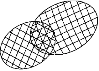
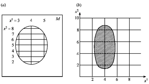
Figure 2.7. (a) A manifoldM, part of the surface of this page, with a coordinate patch. (b) Part ofR
2, showing the coordinate values used in (a).
to remain differentiable at leastntimes after a change of coordinates, at least the firstn derivatives of all the transformation functions must exist. If they do, then we have what is called aCn manifold. Intuitively, we might think it possible to define functions of space and time that can be differentiated any number of times, for which we would needn = ∞. We shall indeed take aC∞manifold as the basis for our model spacetime. Mathematically, though, this is a rather strong assumption, and for many physical purposes it would be sufficient to take, say, n=4.
2.1.3 Summary and examples
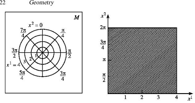
Figure 2.8.Same as figure 2.7, but using different coordinates.
The following examples illustrate, in terms of two-dimensional manifolds, some of the important ideas. Figure 2.7(a) shows a manifold,M, which is part of the surface of the paper on which it is printed. For the sake of argument, I am asking readers to suppose that this surface is perfectly smooth, rather than being composed of tiny fibres. For the definitions to work, we must take the manifold to be the interior of the rectangular region, excluding points on the boundary. The interior of the roughly circular region is a coordinate patch. Inside it are drawn some of the grid lines by means of which we assign coordinatesx1 andx2 to each point. Figure 2.7(b) is a pictorial representation of part of the space R
2 of pairs of coordinates. The interior of the shaded region represents
the coordinates actually used. To every point of this region there corresponds a point of the coordinate patch inM andvice versa. Figure 2.8 shows a similar arrangement, using a different coordinate system. Here, again, theinteriorof the shaded region ofR
2 represents the open set of points that correspond uniquely
to points of the coordinate patch. As before, the boundary of the coordinate patch and the corresponding line x1 = 4 inR
2 are excluded. Also excluded,
however, are the boundary linesx1 = 0, x2 = 0 and x2 = 2π inR
2, which
means that points on the line labelled byx2 =0 in M do not, in fact, belong to the coordinate patch. Since the coordinate system is obviously usable, even when these points are included, their exclusion may seem like an annoying piece of bureaucracy: however, it is essential to apply the rules correctly if the definitions of continuity and differentiability are to work smoothly. For example, the function g(x1,x2)= x2is continuous throughoutR
2, but the corresponding function on
Mis discontinuous atx2=0.
no single patch of any kind could cover all of it. These examples also illustrate the fact that, although the coordinates which label the points ofM have definite numerical values, these values do not, in themselves, supply any notion of a distance between two points. The distance along some curve inM maybe defined by some suitable rule, such as (i) ‘use a ruler’ or (ii) ‘measure the volume of ink used by a standard pen to trace the curve’ or, given a particular coordinate system, (iii) ‘use the mathematical expression D = (function of coordinates)’. Any such rule imposes an additional structure—called a metric—which is not inherent in the manifold. In particular, there is no naturally occurring function for use in (iii). Any specific function, such as the Pythagoras expression, would have quite different effects when applied to different coordinate systems, and the definition of the manifold certainly does not single out a special coordinate system to which that function would apply. We do have a more or less unambiguous means of determining distances on a sheet of paper, and this is because the paper, in addition to the topological properties it possesses as a manifold, has physical properties that enable us to apply a definite measuring procedure. The same is true of space and time and, although we have made some initial assumptions about their topological structure, we have yet to find out what physical properties determine their metrical structure.
2.2
Tensors
From our discussion so far, it is apparent that coordinate systems can be dangerous, even though they are often indispensable for giving concrete descriptions of a physical system. We have seen that the topology of a manifold such as that of space and time may permit the use of a particular coordinate system only within a small patch. Suppose, for the sake of argument, that the surface of the Earth is a smooth sphere. We encounter no difficulty in drawing, say, the street plan of a city on a flat sheet of paper using Cartesian coordinates, but we should obviously be misled if we assumed that this map could be extended straightforwardly to cover the whole globe. By assuming that two-dimensional Euclidean geometry was valid on the surface of the Earth, we should be making a mistake, owing to the curvature of the spherical surface, but the mistake would not become apparent as long as we made measurements only within a region the size of a city. Likewise, physicists before Einstein assumed that a frame of reference fixed on the Earth would be inertial, except for effects of the known orbital motion of the Earth around the Sun and its rotation about its own axis, which could be corrected for if necessary. According to Einstein, however, this assumption is also mistaken. It fails to take account of the true geometry of space and time in much the same way that, by treating a city plan as a Euclidean plane, we fail to take account of the true geometry of the Earth. The mistake only becomes apparent, however, when we make precise observations of gravitational phenomena.
which, we believe, applies to inertial frames. If we do not know,a priori, what the true geometry of space and time is, then we do not know whether any given frame is truly inertial. Therefore, we need to express our laws in a way that does not rely on our making any special assumption about the coordinate system. There are two ways of achieving this. The method adopted by Einstein himself is to write our equations in a form that applies toanycoordinate system: the mathematical tech-niques for doing this constitute what is calledtensor analysis. The other, more recent method is to write them in a manner that makes no reference to coordi-nate systems at all: this requires the techniques ofdifferential geometry. For our purposes, these two approaches are entirely equivalent, but each has its own ad-vantages and disadad-vantages in terms of conceptual and notational clarity. So far as I can, I will follow a middle course, which seems to me to maximize the ad-vantages. Both techniques deal with objects calledtensors. Tensor analysis, like elementary vector analysis, treats them as being defined by sets of components, referred to particular coordinate systems. Differential geometry treats them as entities in their own right, which may be described in terms of components, but need not be. When components are used, the two techniques become identical, so there is no difficulty in changing from one description to the other.
Many, though not all, of the physical objects that inhabit the spacetime manifold will be described by tensors. Atensor at a point P of the manifold refers only to that point. A tensor field assigns some property to every point of the manifold, and most physical quantities will be described by tensor fields. (For brevity, I shall often follow custom by referring to a tensor field simply as a ‘tensor’, when the meaning is obvious from the context.) Tensors and tensor fields are classified by theirrank, a pair of numbersa
b
.
Rank00 tensors, also calledscalars, are simply real numbers. A scalar fieldis a real-valued function, say f(P), which assigns a real number to each point of the manifold. If our manifold were just the three-dimensional space encountered in Newtonian physics, then at a particular instant in time, an electric potentialV(P)or the density of a fluidρ(P)would be examples of scalar fields. In relativistic physics, these and all other simple examples I can think of are not true scalars, because their definitions depend in one way or another on the use of specific coordinate systems or on metrical properties of the space that our manifold does not yet possess. For the time being, however, no great harm will be done if readers bear these examples in mind. If we introduce coordinatesxµ, then we can express f(P)as an algebraic function f(xµ). (For convenience, I am using the same symbol f to denote two different, though related functions: we have f(xµ)= f(P)whenxµare the coordinates of the pointP.) In a different coordinate system, whereP has the coordinatesxµ′, the same quantity will be described by a new algebraic function f′(xµ′), related to the old one by
f′(xµ′)= f(xµ)= f(P). (2.9)
Rank10tensors are calledvectorsin differential geometry. They correspond to what are called contravariant vectors in tensor analysis. The prototypical vector is the tangent vector to a curve. In ordinary Euclidean geometry, the equation of a curve may be expressed parametrically by giving three functions x(λ),y(λ)andz(λ), so that each point of the curve is labelled by a value ofλ
and the functions give its coordinates. Ifλ is chosen to be the distance along the curve from a given starting point, then the tangent vector to the curve at the point labelled byλ has components(dx/dλ,dy/dλ,dz/dλ). In our manifold, we have not yet given any meaning to ‘distance along the curve’, and we want to avoid defining vectors in terms of their components relative to a specific coordinate system. Differential geometry provides the following indirect method of generalizing the notion of a vector to any manifold. Consider, in Euclidean space, a differentiable function f(x,y,z). This function has, in particular, a value f(λ)at each point of the curve, which we obtain by substituting forx,yandzthe appropriate functions ofλ. The rate of change of f with respect toλis
df component of the tangent vector. All the information about the tangent vector is contained in the differential operator d/dλ, and in differential geometry this operator is defined tobethe tangent vector.
A little care is required when applying this definition to our manifold. We can certainly draw a continuous curve on the manifold and label its points continuously by a parameter λ. What we cannot yet do is select a special parameter that measures distance along it. Clearly, by choosing different parametrizations of the curve, we shall arrive at different definitions of its tangent vectors. It is convenient to refer to the one-dimensional set of points in the manifold as apath. Then each path may be parametrized in many different ways, and we regard each parametrization as a distinctcurve. This has the advantage that each curve, with its parameterλ, has a unique tangent vector d/dλat every point. Suppose we have two curves, corresponding to the same path, but with parametersλandµthat are related byµ=aλ+b,aandbbeing constants. The difference is obviously a rather trivial one and the two parameters are said to be affinely related.
lower indices, and repeated indices implying a sum may both appear in the same position.) I shall use bold capital letters to denote vectors, such asV = d/dλ. If, then, a curve is represented in a particular coordinate system by the functions xµ(λ), we can write
where the partial derivativesXµ=∂/∂xµare identified as the basis vectors in this system andVµare the corresponding components ofV. Note that components of a vector are labelled by upper indices and basis vectors by lower ones. In a new coordinate system, with coordinatesxµ′, and basis vectorsXµ′ = ∂/∂xµ
µ′ shows that the same vector has components
Vµ′ =∂x µ′
∂xµV µ.
(2.12)
In tensor analysis, a contravariant vector is defined by specifying its components in some chosen coordinate system and requiring its components in any other system to be those given by the transformation law (2.12). It will be convenient to denote the transformation matrix by
µµ′ = ∂x µ′
∂xµ. (2.13)
The convention of placing a prime on the indexµ′ to indicate thatxµandxµ′ belong to different coordinate systems, rather than writing, say,x′µ, is useful here in indicating to which system each index onrefers. Using the chain rule again, we find
Rank01tensors are calledone-formsin differential geometry orcovariant vectorsin tensor analysis. Consider the scalar product u·v of two Euclidean vectors. Normally, we regard this product as a rule that combines two vectors uandvto produce a real number. As we shall see, this scalar product involves metrical properties of Euclidean space that our manifold does not yet possess. There is, however, a different point of view that can be transferred to manifold. For a given vector u, the symbol u· can be regarded as defining a function, whose argument is a vector, say v, and whose value is the real numberu ·v. The functionu·is linear. That is to say, if we give it the argumentav+bw, wherevandware any two vectors, anda andbare any two real numbers, then
is a vector:ω(V)=(real number). Because the one-form is a linear function, its value must be a linear combination of the components of the vector:
ω(V)=ωµVµ. (2.15)
The coefficientsωµare the components of the one-form, relative to the coordinate system in whichV has componentsVµ. Aone-form fieldis defined in the same way as a linear function of vector fields, whose value is a scalar field. In the definition of linearity,aandbmay be any two scalar fields.
The expression (2.15) is, of course, similar to the rule for calculating the scalar product of two Euclidean vectors from their components. Nevertheless, it is clear from their definitions that vectors and one-forms are quite different things, and (2.15) does not allow us to form a scalar product of two vectors.
An example of a one-form field is the gradient of a scalar field f, whose components are ∂µf. Notice the consistency of the convention for placing indices: the components of a one-form have indices that naturally appear in the lower position. Call this gradient one-formωf. IfV =d/dλis the tangent vector to a curvexµ(λ), then the new scalar fieldωf(V)is the rate of change of f along
Since vectors and one-forms exist independently of any coordinate system, the function ω(V) given in (2.15) must be a true scalar field—it must have the same value in any coordinate system. This means that the matrix which transforms the components of a one-form between two coordinate systems must be the inverse of that which transforms the components of a vector:
ωµ′ =ωµµ
In tensor analysis, a covariant vector is defined by requiring that its components obey the transformation law (2.17). Clearly, this is indeed the correct way of transforming a gradient.
Ranka b
the components are then given by a transformation law that generalizes those for vectors and one-forms in an obvious way:
Tα′β′...µ′ν′...=α ′ α
β′ β· · ·
µ
µ′νν′· · ·Tαβ...µν.... (2.19)
From this we can see how to construct laws of physics in a way that will make them true in any coordinate system. Suppose that a fact about some physical system is expressed in the formS = T, whereS andT are tensors of the same rank. On multiplying this equation on both sides by the appropriate product of
matrices, we obtain the equationS′ = T′, which expresses the same fact, in an equation of the same form, but now applies to the new coordinate system. The point that may require some effort is to make sure thatSandT reallyaretensors that transform in the appropriate way.
Ifωis a one-form and V a vector, then thed2quantities Tν
µ = ωµVν are the components of a rank11tensor. As we saw in (2.15), by settingµ=νand carrying out the implied sum, we obtain a single number, which is a scalar (or a rank00tensor). This process is calledcontraction. Given any tensor of rankab, witha≥1 andb≥1, we may contract an upper index with a lower one to obtain a new tensor of ranka−b−11. Readers should find it an easy matter to check from (2.19) that, for example, the objectSαγ ...ν... = T
αβγ ...
βν...does indeed transform in the right way.
2.3
Extra Geometrical Structures
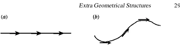
Figure 2.9.(a) A geodesic curve: successive tangent vectors are parallel to each other. (b) A non-geodesic curve: successive tangent vectors are not parallel.
2.3.1 The affine connection
There are four important geometrical tools provided by an affine connection: the notion ofparallelism, the notion ofcurvature, thecovariant derivativeand the geodesic. Let us first understand what it is good for.
a) Newton’s first law of motion claims that ‘a body moves at constant speed in a straight line unless it is acted on by a force’. In general relativity, we shall replace this with the assertion that ‘a test particle follows a geodesic curve unless it is acted on by a non-gravitational force’. As we saw earlier, gravitational forces are going to be interpreted in terms of spacetime geometry, which itself is modified by the presence of gravitating bodies. By a ‘test particle’, we mean one that responds to this geometry, but does not modify it significantly. Ageodesicis a generalization of the straight line of Euclidean geometry. It is defined, roughly, as a curve whose tangent vectors at successive points are parallel, as illustrated in figure 2.9. Given a definition of ‘parallel’, as provided by the connection, this is perhaps intuitively recognizable as the natural state of motion for a particle that is not disturbed by external influences.
b) The equations of physics, which we wish to express entirely in terms of tensors, frequently involve the derivatives of vector or tensor fields. Now, the derivatives of a scalar field∂µf are, as we have seen, the components of a one-form field. However, the derivatives of the components of a vector field,
∂µVν, are not the components of a tensor field, even though they are labelled by a contravariant and a covariant index. On transforming these derivatives to a new coordinate system, we find
∂µ′Vν ′
=µµ′∂µ(ν ′ νVν)
=µµ′ν ′
ν∂µVν+µµ′(∂µν ′
ν)Vν. (2.20)
Because of the last term, this does not agree with the transformation law for a second-rank tensor. The affine connection will enable us to define what is called acovariant derivative,∇µ, whose action on a vector field is of the form ∇µVν = ∂µVν + (connection term). The transformation of the extra term involving the affine connection will serve to cancel the unwanted part in (2.20), so that∇µVνwill be a tensor.
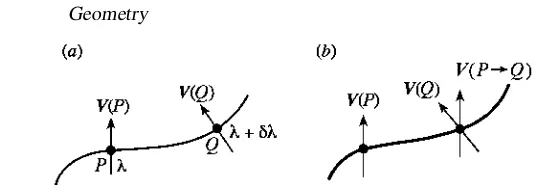
Figure 2.10.V(P)andV(Q)are the vectors atPandQbelonging to the vector fieldV.
V(P →Q)is the vector atQwhich results from parallelly transportingV(P)along the curve.
goes wrong, consider the derivative of a component of a vector field along a curve, as illustrated in figure 2.10(a), where P and Q are points on the curve with parametersλandλ+δλrespectively. The derivative atPis
dVµ dλ =
dxν dλ
∂Vµ
∂xν =δλlim→0
Vµ(Q)−Vµ(P)
δλ . (2.21)
For a scalar field, which has unique values at P andQ, such a derivative makes good sense. However, the values at P and Q of the components of a vector field depend on the coordinate system to which they are referred. It is easy to make a change of coordinates such that, for example,Vµ(Q)is changed while Vµ(P)is not, and so the difference of these two quantities has no coordinate-independent meaning. If we try to find the derivative of the vector field itself, we shall encounter the expressionV(Q)−V(P). Now, V(P)is the tangent vector to some curve passing throughP(though not necessarily the one shown in figure 2.10(a)) andV(Q)is the tangent vector to some curve passing throughQ. The difference of two vectors atPis another vector at P: each vector is tangent to some curve passing throughP. However,V(Q)−V(P)is not, in general, the tangent vector to a curve at a specific point. It is not, therefore, a vector and has, indeed, no obvious significance at all.
To define a meaningful derivative of a vector field, we need to compare two vectors at the same point, say Q. Therefore, we construct a new vector V(P →Q), which exists atQbut representsV(P). Then a new vector, DV/dλ, which will be regarded as the derivative ofValong the curve, may be defined as
DV dλ
P
= lim δλ→0
V(Q)−V(P→ Q)
δλ . (2.22)
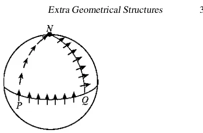
Figure 2.11. Parallel transport of a vector from P toQ on a spherical surface by two routes.
connectiondefineswhat it means for a vector atQto be parallel to one atP: it is said to defineparallel transportof a vector along the curve. From a mathematical point of view, we are free to specify the affine connection in any way we choose. Physically, on the other hand, we shall need to find out what the affine connection is, with which nature has actually provided us, and we shall address this problem in due course. It might be thought that a vector which representsV(P)should not only be parallel to it but also have the same length. In Euclidean geometry, the magnitude of a vector is(v ·v)1/2and, as we have seen, the scalar product needs a metric for its definition. The metric connection, mentioned above, does indeed define parallel transport in a manner that preserves the magnitude of the transported vector.
The concrete definition of parallel transport is most clearly written down by choosing a coordinate system. IfPandQlie on a curvexµ(λ)and are separated by an infinitesimal parameter distanceδλ, then the components ofV(P → Q)
are defined by
Vµ(P→ Q)=Vµ(P)−δλŴµνσ(P)Vν(P)dx
σ
dλ (2.23)
The idea of parallel transport is illustrated in figure 2.11, which shows the surface of a Euclidean sphere. For the purposes of this example, we assume the usual metrical properties of Euclidean space, so that distances and angles have their usual meanings. The manifold we consider is the two-dimensional surface of the sphere, so every vector is tangential to this surface.PandQare points on the equator, separated by a quarter of its circumference, andN is the north pole. The equator and the curvesP N andQ N are parts of great circles on the sphere and are ‘straight lines’ as far as geometry on the spherical surface is concerned: one would follow such a path by walking straight ahead on the surface of a perfectly smooth Earth. Consider a vector V(P)that points due north—it is a tangent vector at Pto the curveP N. We shall transport this vector to Q, first along the equator and second via the north pole. The rule for parallel transport of a vector along a straight line is particularly simple: the angle between the vector and the line remains constant. For transport along the equator, the vector clearly points north at each step and soV(P → Q)also points north alongQ N. Along P N, the vector also points north, so on arrival at the pole it is perpendicular to Q N. On its way south, it stays perpendicular to Q N. Thus, the transported vector V(P →Q)as defined by the polar route points along the equator.
At this point, readers should consider parallel transport along the sides of a plane equilateral triangle P N Q. It is easy to see that V(P → Q) is independent of the route taken. Clearly, the difference between the two cases is that the spherical surface is curved while the plane surface is flat. The rule for parallel transport, embodied mathematically in the affine connection coefficients, evidently provides a measure of the curvature of a manifold, and we shall later formulate this precisely. It should be emphasized that a manifold possesses a curvatureonly whenit has an affine connection. If it has no connection, then it is neither curved nor flat: the question just does not arise. Finally, returning to figure 2.11, suppose that we had chosenQto lie close toP and considered only paths contained in a small neighbourhood of the two points. The surface would have been almost indistinguishable from a flat one and the transported vector would have been almost independent of the path. This is consistent with the mathematical expression (2.23). IfPhas coordinatesxµandQis infinitesimally close toP, with coordinatesxµ+dxµ, then we may substitute dxµforδλdxµ/dλ, and all reference to the path betweenPandQdisappears. The affine connection of two-dimensional Euclidean geometry is explored in exercise 2.10.
One of our motivations for introducing the affine connection was to be able to define a meaningful derivative of a vector field. The covariant derivative along a curve was to be defined, using the idea of parallel transport, by (2.22). As we have just seen, it is not actually necessary to specify a curve when P and Q are infinitesimally close. In terms of components, then, let us write DVµ/dλ= (dxσ/dλ)∇σVµ and calculate the covariant derivative∇σVµ using (2.22) and (2.23). We find
Notice that the three indices of the connection coefficient have different functions. There are, indeed, important situations in which the connection issymmetricin its two lower indices:Ŵµνσ =Ŵµσ ν. In general, however, it is the last index that corresponds to that of∇σ. Since DVµ/dλand dxσ/dλare both vectors, it follows from their transformation laws that the functions∇σVµare the components of a rank1
From this, we can deduce the transformation law for the connection coefficients themselves, which can be written as
Readers are urged to verify this in detail, bearing in mind that∂σ′(µ ′
Evidently, the affine connection is not itself a tensor. However, the covariant derivative that contains it acts on any tensor to produce another tensor of one higher covariant rank. So far, we have defined only the covariant derivative of a vector field, which was given in (2.24). The covariant derivative of a scalar field is just the partial derivative,∇µf =∂µf, since this is already a vector field. In order for the covariant derivative of a one-form field to be a second-rank tensor field, we must have
∇σωµ=∂σωµ−Ŵνµσων. (2.27)
Notice that the roles of the upper and first lower indices have been reversed, compared with (2.24), and that the sign of the connection term has changed. It is straightforward to check that these changes are vital if this derivative is to transform as a rank0
2
tensor field. The covariant derivative of a tensor field of arbitrary rank is
∇σTαβ...µν...=∂σTαβ...µν...+(connection terms). (2.28)
There is one connection term for each index of the original tensor. For each upper index, it is a term like that in (2.24) and for each lower index it is like that in (2.27). Exercise 2.11 invites readers to consider in more detail how these definitions are arrived at.
There is a convenient notation that represents partial derivatives of tensor fields by a comma and covariant derivatives by a semicolon. That is:
∂σTαµν≡Tαµν,σ and ∇σTαµν≡Tαµν;σ. (2.29)
2.3.2 Geodesics
of straight lines that make sense in our manifold with its affine connection. For example, the idea that a straight line is the shortest distance between two points will make sense only when we have a metric to measure distances. The idea of a geodesic is that, if we are to walk along a straight line, each step we take must be parallel to the last. Consider, then, the special case of the parallel transport equation (2.23) in which the vector transported fromP toQ is the curve’s own tangent vector atP: Vµ = dxµ/dλ. If the curve is a geodesic, the transported vector V(P → Q)will be proportional to V(Q). Since the vectors have no definite length, the constant of proportionality may well depend on λ, but if P and Q are separated by an infinitesimal parameter distance, it will be only infinitesimally different from 1. So we may write
dxµ
where f(λ) is an unknown function. Using this in (2.23) and taking the limit
δλ→0, we obtain thegeodesic equation
d2xµ
A curvexµ(λ)is a geodesic if and only if it satisfies an equation of this form, where f(λ)can be any function.
Remember now that a given path through the manifold can be parametrized in many different ways, each one being regarded as a different curve. It is easy to see that if the curve given by one parametrization is a geodesic, then so is the curve that results from another parametrization of the same path. We need only express the new parameter, sayµ, as a function of λand use the chain rule in (2.31):
This has the same form as (2.31) but involves a different function ofµon the right-hand side. In particular, it is always possible to find a parameter for which the right-hand side of (2.32) vanishes. Such a parameter is called anaffine parameter for the path. It is left as a simple exercise for the reader to show that ifλis an affine parameter, then any parameter that is affinely related to it (that is, it is a linear functionµ=aλ+b) is also an affine parameter.
2.3.3 The Riemann curvature tensor
Figure 2.12.Two paths,P R QandP S Q, for parallelly transporting a vector fromPtoQ.
connection. The definition of curvature is made precise by the Riemann curvature tensor. Consider two points P and Q with coordinates xµ and xµ + δxµ respectively, such thatδxµ =0, except forµ=1 or 2. A region of the(x1,x2)
surface near these points is shown in figure 2.12. By transporting a vectorV(P)
to Q via R or S, we obtain at Q the two vectors V(P → R → Q) and V(P → S → Q). To first order in δxµ these two vectors are the same, as we have seen. If we expand them to second order, however, they are different, and we obtain an expression of the form
Vµ(P →S →Q)−Vµ(P → R→ Q)=Rµν12Vνδx1δx2+. . . (2.33)
where the quantities Rµν12 depend on the connection coefficients and their derivatives. Readers are invited to verify that they are components of the Riemann tensor we are about to define.
It should be clear that the process of transporting the vector from P to Q along the two paths is related to that of taking two derivatives, with respect tox1 andx2, in either order. If we act on a vector field with the two covariant derivatives ∇σ and∇τ in succession, the result depends on the order of the two operations; they do not commute. To work out the commutator, we use the definition (2.28), bearing in mind that∇σVµis itself a rank11tensor. The result is
[∇σ,∇τ]Vµ≡ ∇σ∇τVµ− ∇τ∇σVµ= Rµνσ τVν+Ŵλσ τ −Ŵλτ σ∇λVµ (2.34) where
Rµνσ τ =Ŵµντ,σ−Ŵµνσ,τ +ŴµλσŴλντ−ŴµλτŴλνσ. (2.35)