LAMPIRAN A
HASIL UJI MUTU FISIK SERBUK Mutu Fisik
yang Diuji
HASIL UJI DENSITAS SERBUK Mutu Fisik
yang Diuji
Rep. Uji Formula Tablet Ibuprofen Persyarat an F I F II F III F IV
Densitas (g/ml)
I bulk 0,3924 0,6295 0,3550 0,6141
- tapped 0,4905 0,7153 0,4438 0,6978
II bulk 0,4035 0,6391 0,3761 0,6122 tapped 0,5044 0,7263 0,4643 0,6879 II bulk 0,4135 0,6593 0,3982 0,6228 tapped 0,5105 0,7492 0,4978 0,6998
x
bulk 0,4031 0,6426 0,3764 0,6164 SD bulk 0,01 0,02 0,02 0,00LAMPIRAN B
HASIL UJI KESERAGAMAN BOBOT TABLET IBUPROFEN
Replikasi I
No. Bobot Tablet Ibuprofen (mg)
F I F II F III F IV
1. 803,3 804,2 771,3 791,8
2. 802,8 800,4 771,9 785,3
3. 809,3 802,7 772,0 791,0
4. 808,0 805,8 775,7 789,8
5. 797,1 803,8 779,5 783,9
6. 805,7 802,6 781,7 795,2
7. 803,1 800,5 774,6 794,2
8. 799,3 804,3 776,0 802,0
9. 799,6 805,9 773,5 794,2
10. 801,2 803,3 788,0 783,5
11. 806,8 804,7 771,3 782,6
12. 797,4 801,8 776,4 786,3
13. 791,6 803,6 774,5 794,9
14. 803,9 803,4 786,5 800,7
15. 798,2 801,9 774,3 786,5
16. 795,2 799,6 776,5 788,6
17. 808,0 803,4 771,3 784,5
18. 794,5 800,8 782,3 794,4
19. 801,2 803,9 783,6 795,3
20. 797,5 803,0 779,1 791,4
x
801,19 802,98 777,00 790,81SD 4,92 1,73 5,12 5,62
Replikasi II
No. Bobot Tablet Ibuprofen (mg)
F I F II F III F IV
1. 807,0 807,8 771,5 792,8
2. 808,3 806,0 783,9 796,7
3. 801,6 807,7 770,0 793,0
4. 802,4 809,5 771,7 797,3
5. 807,6 810,4 776,4 795,0
6. 806,7 808,4 789,9 794,3
7. 805,1 807,0 771,2 793,0
8. 800,3 811,3 771,8 790,0
9. 800,5 812,6 771,5 800,5
10. 805,5 810,4 777,9 794,4
11. 802,7 811,1 772,1 801,1
12. 804,5 809,9 776,3 795,1
13. 803,0 808,1 776,9 795,4
14. 806,6 806,6 773,6 800,9
15. 802,7 810,7 770,5 794,6
16. 805,1 811,6 787,0 796,2
17. 801,3 807,6 775,7 796,4
18. 804,0 809,9 778,0 800,2
19. 803,7 810,7 773,1 796,8
20. 804,7 811,0 771,1 800,9
x
804,17 809,42 775,51 796,23SD 2,36 1,87 5,62 3,14
Replikasi III
No. Bobot Tablet Ibuprofen (mg)
F I F II F III F IV
1. 800,8 800,1 795,9 797,4
2. 805,1 796,9 779,9 797,7
3. 798,6 799,6 788,3 795,6
4. 796,6 793,0 791,8 794,8
5. 803,1 803,0 793,9 799,2
6. 805,3 797,8 787,5 793,3
7. 789,5 793,8 786,5 798,3
8. 791,4 801,2 794,5 801,9
9. 793,4 796,8 787,3 799,1
10. 800,7 799,5 789,6 800,5
11. 799,1 793,0 788,9 799,6
12. 800,3 802,8 800,1 798,2
13. 798,8 800,7 791,7 797,8
14. 798,2 800,0 790,4 800,0
15. 800,7 792,0 788,1 797,5
16. 803,4 795,4 794,0 798,1
17. 794,9 803,6 800,2 799,1
18. 802,9 804,6 790,4 798,6
19. 795,3 797,1 794,8 795,9
20. 793,0 795,0 778,1 794,2
x
798.56 798,30 790,60 797,84SD 4,52 3,80 5,58 2,17
LAMPIRAN C
HASIL UJI KEKERASAN TABLET IBUPROFEN
Replikasi I
No. Kekerasan Tablet Ibuprofen (Kgf)
F I F II F III F IV
No. Kekerasan Tablet Ibuprofen (Kgf)
Replikasi III
No. Kekerasan Tablet Ibuprofen (Kgf)
F I F II F III F IV
1. 13,0 11,9 12,2 10,5
2. 13,1 12,1 12,3 10,8
3. 13,7 11,6 12,4 11,0
4. 13,2 12,0 12,0 11,0
5. 13,3 12,4 11,9 10,7
6. 13,6 11,9 12,4 10,8
7. 13,4 12,1 12,0 10,5
8. 13,6 12,3 11,9 10,6
9. 13,5 11,8 12,2 10,7
10. 13,1 12,1 12,3 10,9
x
13,35 12,02 12,16 10,75LAMPIRAN D
HASIL UJI KERAPUHAN TABLET IBUPROFEN
LAMPIRAN E
HASIL UJI WAKTU HANCUR TABLET IBUPROFEN
Replikasi Waktu Hancur (detik)
F I F II F III F IV
1 12 26 9 28
2 11 39 8 26
3 8 24 10 21
X 10,33 29,67 9,00 25,00
LAMPIRAN F
HASIL UJI PENETAPAN KADAR TABLET IBUPROFEN
LAMPIRAN G
HASIL UJI DISOLUSI TABLET IBUPROFEN PADA t = 30 MENIT
LAMPIRAN H
CONTOH PERHITUNGAN SUDUT DIAM
Formula I:
CONTOH PERHITUNGAN INDEKS KOMPRESIBILITAS Formula I :
% kompresibilitas = 100%
CONTOH PERHITUNGAN AKURASI DAN PRESISI Formula I replikasi 1
Absorbansi = 0,680 y = 0,0017x + 0,0024 Konsentrasi Sampel (x) = 405,6203 g/ml Berat teoritis = 0,3200 gram
CONTOH PERHITUNGAN UJI PENETAPAN KADAR Formula I replikasi 1
Absorbansi = 0,838 y = 0,0017x + 0,0024 Konsentrasi sampel (x) = 500,2012 g/ml Berat tablet = 0,8000 gram
Berat teoritis = 0,8000 x 0,4 = 0,4000 gram 0,8
Konsentrasi teoritis = 0,4000 x 106 x 1,25 = 500 g/ml 100 10
% perolehan kembali = konsentrasi sampel x 100 % konsentrasi teoritis
CONTOH PERHITUNGAN PERSEN OBAT TERLEPAS Formula I replikasi 1
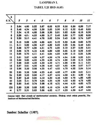
LAMPIRAN I
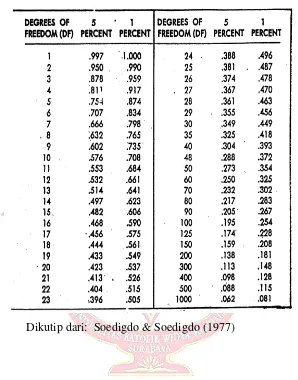
LAMPIRAN K TABEL UJI r
LAMPIRAN N
HASIL UJI STATISTIK KEKERASAN TABLET IBUPROFEN ANTAR FORMULA Interval for Mean
Min Max
Multiple Comparisons Kekerasan tablet
HSD
* The mean difference is significant at the 0,05 level. Keterangan:
LAMPIRAN O
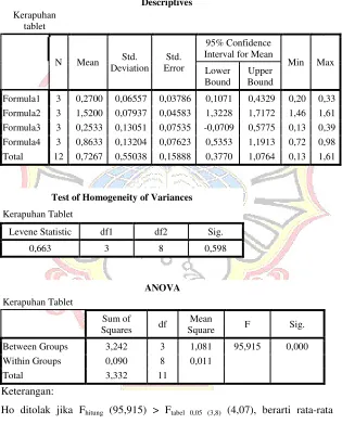
HASIL UJI STATISTIK KERAPUHAN TABLET IBUPROFEN ANTAR FORMULA Interval for Mean
Min Max
Test of Homogeneity of Variances
Multiple Comparisons
*. The mean difference is significant at the 0.05 level. Keterangan:
LAMPIRAN P
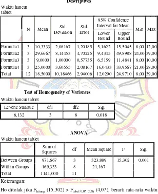
HASIL UJI STATISTIK WAKTU HANCUR TABLET IBUPROFEN ANTAR FORMULA Interval for Mean
Min Max
Test of Homogeneity of Variances Waktu hancur tablet
Levene Statistic df1 df2 Sig.
6,132 3 8 0,018
ANOVA Waktu hancur tablet
Sum of
Multiple Comparisons
Waktu hancur tablet HSD
Formula1 19,33333* 3,75648 0,001 10,6709 27,9958
Formula3 20,66667* 3,75648 0,001 12,0042 29,3291
Formula4 4,66667 3,75648 0,249 -3,9958 13,3291
Formula1 14,66667* 3,75648 0,005 6,0042 23,3291
Formula2 -4,66667 3,75648 0,249 -13,3291 3,9958
Formula3 16,00000* 3,75648 0,003 7,3376 24,6624
*. The mean difference is significant at the 0.05 level. Keterangan:
LAMPIRAN Q
HASIL UJI STATISTIK DISOLUSI TABLET IBUPROFEN ANTAR FORMULA
Deviation Std. Error
95% Confidence Interval for Mean
Min Max
Test of Homogeneity of Variances
Persen obat terlarut
Levene Statistic df1 df2 Sig.
1.058 3 8 0,419
ANOVA Persen obat terlarut
Sum of
Multiple Comparisons
Persen obat terlarut HSD
*. The mean difference is significant at the 0.05 level. Keterangan:
LAMPIRAN R
HASIL UJI STATISTIK PENETAPAN KADAR TABLET IBUPROFEN ANTAR FORMULA
Descriptives Interval for Mean
Min Max
Test of Homogeneity of Variances
Kadar tablet ibuprofen
Levene Statistic df1 df2 Sig.
0,513 3 8 0,685
ANOVA Kadar tablet ibuprofen
LAMPIRAN S
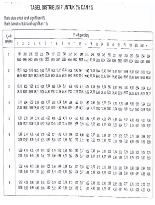
UJI F KURVA BAKU DENGAN NaOH 0,1N UNTUK UJI PENETAPAN KADAR TABLET IBUPROFEN
Rep. Konsentrasi (ppm) (x) 2095,8 3,542 906363,64 2,563276 1523,946 Persamaan Regresi pada replikasi 1 y = 0,0016x + 0,0157
rhitung/rtabel: ,9993/0,811
Rep. Konsentrasi (ppm) (x) 400,4 0,682 160320,16 0,465124 273,0728 500,5 0,838 250500,25 0,702244 419,4190 600,6 0,993 360720,36 0,986049 596,3958 2102,1 3,534 911820,91 2,565498 1529,2277 Persamaan Regresi pada replikasi 2 y = 0,0017x + 0,0074
Rep. Konsentrasi 399,6 0,678 159680,16 0,459684 270,9288 499,5 0,837 249500,25 0,700569 418,0815 599,4 0,996 359280,36 0,992016 597,0024 2097,9 3,519 908180,91 2,551605 1522,1763 Persamaan Regresi pada replikasi 3 y = 0,0017x + 0,0024
rhitung/rtabel: 0,9997/0,811
x2 xy y2 n Residual
regression 0,002073527 12
Common
regression 2726365,46 4575,3500 7,680379 0,002087909 15
Fhitung = 0,027742993 F tabel 0,05 (3,12) = 3,49
LAMPIRAN T
UJI F KURVA BAKU DENGAN DAPAR FOSFAT 0,2 M pH 7,2 UNTUK UJI DISOLUSI TABLET IBUPROFEN
Rep. Konsentrasi (ppm) (x) 400,4 0,720 160320,16 0,518400 288,2880 500,5 0,909 250500,25 0,826281 454,9545 600,6 1,014 360720,36 1,028196 609,0084 2102,1 3,705 911820,91 2,812563 1600,5990 Persamaan Regresi pada replikasi 1 y = 0,0017x + 0,0130
rhitung/rtabel: 0,9974/0,811
Rep. Konsentrasi (ppm) (x) 400,4 0,722 160320,16 0,521284 289,0888 500,5 0,919 250500,25 0,844561 459,9595 600,6 1,092 360720,36 1,192464 655,8552 2102,1 3,823 911820,91 3,020955 1659,6580 Persamaan Regresi pada replikasi 2 y = 0,0018x - 0,0027
Rep. Konsentrasi 400,8 0,721 160640,64 0,519841 288,9768 501,0 0,912 251001,00 0,831744 456,9120 601,2 1,090 361441,44 1,188100 655,3080 2104,2 3,816 913643,64 3,007850 1657,7088 Persamaan Regresi pada replikasi 3 y = 0,0018x - 0,0016
rhitung/rtabel: 0,999904/0,811
x2 xy y2 n Residual
regression 0,003121451 12
Common
regression 2737285,46 4917,9658 8,841368 0,005465438 15
Fhitung = 3,003715147 F tabel 0,05 (3,12) = 3,49
LAMPIRAN U
HASIL UJI ANAVA KEKERASAN TABLET IBUPROFEN DENGAN DESIGN EXPERT
Use your mouse to right click on individual cells for definitions.
Response 1 Kekerasan
ANOVA for selected factorial model
Analysis of variance table [Partial sum of squares - Type III]
Source Sum of
Squares
df Mean Square
F Value p-value Prop > F
Model 27.41 3 9.14 15.20 0.0011 significant
A-Macam filler-binder 19.71 1 19.71 32.80 0.0004
B-Macam superdisintegrant 7.49 1 7.49 12.46 0.0077
AB 0.21 1 0.21 0.35 0.5678
Pure Error 4.81 8 0.60
Cor Total 32.22 11
The Model F-value of 15.20 implies the model is significant. There is only a 0.11% chance that a "Model F-Value" this large could occur due to noise. Values of "Prob > F" less than 0.0500 indicate model terms are significant. In this case A, B are significant model terms.
Values greater than 0.1000 indicate the model terms are not significant.
Std. Dev. 0.78 R-Squared 0.8508
Mean 12.26 Adj R-Squared 0.7948
C.V. % 6.32 Pred R-Squared 0.6643
PRESS 10.82 Adeq Precision 9.257
The "Pred R-Squared" of 0.6643 is in reasonable agreement with the "Adj R-Squared" of 0.7948.
"Adeq Precision" measures the signal to noise ratio. A ratio greater than 4 is desirable. Your ratio of 9.257 indicates an adequate signal. This model can be used to navigate the design space.
Factor Coefficient
Estimate
df Standard Error
95% CI Low
95% CI High
VIF
Intercept 12.26 1 0.22 11.75 12.78
A-Macam filler-binder -1.28 1 0.22 -1.80 -0.27 1.00
B-Macam superdisintegrant -0.79 1 0.22 -1.31 -0.27 1.00
AB 0.13 1 0.22 -0.38 0.65 1.00
Final Equation in Terms of Coded Factors: Kekerasan =
+12.26
-1.28 * A
-0.79 * B
Final Equation in Terms of Actual Factors: Kekerasan =
+12.26167
-1.28167 * Macam filler-binder -0.79000 * Macam superdisintegrant
+0.13333 * Macam filler-binder * Macam superdisintegrant
The Diagnostics Case Statistics Report has been moved to the Diagnostics Node. In the Diagnostics Node, Select Case Statistics from the View Menu.
Proceed to Diagnostic Plots (the next icon in progression). Be sure to look at the:
1) Normal probability plot of the studentized residuals to check for normality of residuals. 2) Studentized residuals versus predicted values to check for constant error.
3) Externally Studentized Residuals to look for outliers, i.e., influential values. 4) Box-Cox plot for power transformations.
LAMPIRAN V
HASIL UJI ANAVA KERAPUHAN TABLET IBUPROFEN DENGAN DESIGN EXPERT
Use your mouse to right click on individual cells for definitions.
Response 2 Kerapuhan
ANOVA for selected factorial model
Analysis of variance table [Partial sum of squares - Type III]
Source Sum of
Squares
df Mean Square
F Value p-value Prop > F
Model 3.24 3 1.08 95.92 < 0.0001 significant
A-Macam filler-binder 2.59 1 2.59 230.30 < 0.0001
B-Macam superdisintegrant 0.34 1 0.34 30.18 0.0006
AB 0.31 1 0.31 27.27 0.0008
Pure Error 0.090 8 0.011
Cor Total 3.33 11
The Model F-value of 95.92 implies the model is significant. There is only a 0.01% chance that a "Model F-Value" this large could occur due to noise. Values of "Prob > F" less than 0.0500 indicate model terms are significant. In this case A, B, AB are significant model terms.
Values greater than 0.1000 indicate the model terms are not significant.
Std. Dev. 0.11 R-Squared 0.9729
Mean 0.73 Adj R-Squared 0.9628
C.V. % 14.61 Pred R-Squared 0.9391
PRESS 0.20 Adeq Precision 20.669
The "Pred R-Squared" of 0.9391 is in reasonable agreement with the "Adj R-Squared" of 0.9628.
"Adeq Precision" measures the signal to noise ratio. A ratio greater than 4 is desirable. Your ratio of 20.669 indicates an adequate signal. This model can be used to navigate the design space.
Factor Coefficient
Estimate
df Standard Error
95% CI Low
95% CI High
VIF
Intercept 0.73 1 0.031 0.66 0.80
A-Macam filler-binder 0.47 1 0.031 0.39 0.54 1.00
B-Macam superdisintegrant -0.17 1 0.031 -0.24 -0.098 1.00
AB -0.16 1 0.031 -0.23 -0.089 1.00
Final Equation in Terms of Coded Factors: Kerapuhan =
+0.73
+0.47 * A
Final Equation in Terms of Actual Factors: Kerapuhan =
+0.72667
+0.46500 * Macam filler-binder -0.16833 * Macam superdisintegrant
-0.16000 * Macam filler-binder * Macam superdisintegrant
The Diagnostics Case Statistics Report has been moved to the Diagnostics Node. In the Diagnostics Node, Select Case Statistics from the View Menu.
Proceed to Diagnostic Plots (the next icon in progression). Be sure to look at the:
1) Normal probability plot of the studentized residuals to check for normality of residuals. 2) Studentized residuals versus predicted values to check for constant error.
3) Externally Studentized Residuals to look for outliers, i.e., influential values. 4) Box-Cox plot for power transformations.
LAMPIRAN W
HASIL UJI ANAVA WAKTU HANCUR TABLET IBUPROFEN DENGAN DESIGN EXPERT
Use your mouse to right click on individual cells for definitions.
Response 3 Waktu hancur
ANOVA for selected factorial model
Analysis of variance table [Partial sum of squares - Type III]
Source Sum of
Squares
Df Mean Square
F Value p-value Prop > F
Model 971.67 3 323.89 15.30 0.0011 significant
A-Macam filler-binder 936.33 1 936.33 44.24 0.0002
B-Macam superdisintegrant 27.00 1 27.00 1.28 0.2914
AB 8.33 1 8.33 0.39 0.5478
Pure Error 169.33 8 21.17
Cor Total 1141.00 11
The Model F-value of 15.30 implies the model is significant. There is only a 0.11% chance that a "Model F-Value" this large could occur due to noise. Values of "Prob > F" less than 0.0500 indicate model terms are significant. In this case A are significant model terms.
Values greater than 0.1000 indicate the model terms are not significant.
Std. Dev. 4.60 R-Squared 0.8516
Mean 18.50 Adj R-Squared 0.7959
C.V. % 24.87 Pred R-Squared 0.6661
PRESS 381.00 Adeq Precision 7.780
The "Pred R-Squared" of 0.6661 is in reasonable agreement with the "Adj R-Squared" of 0.7959.
"Adeq Precision" measures the signal to noise ratio. A ratio greater than 4 is desirable. Your ratio of 7.780 indicates an adequate signal. This model can be used to navigate the design space.
Factor Coefficient
Estimate
df Standard Error
95% CI Low
95% CI High
VIF
Intercept 18.50 1 1.33 15.44 21.56
A-Macam filler-binder 8.83 1 1.33 5.77 11.90 1.00
B-Macam superdisintegrant -1.50 1 1.33 -4.56 1.56 1.00
AB -0.83 1 1.33 -0.39 2.23 1.00
Final Equation in Terms of Coded Factors:
Waktu hancur =
+18.50
+8.83 * A
-1.50 * B
-0.83 * A * B
Final Equation in Terms of Actual Factors:
Waktu hancur =
+18.50000
+8.83333 * Macam filler-binder
-1.50000 * Macam superdisintegrant
-0.83333 * Macam filler-binder * Macam superdisintegrant
The Diagnostics Case Statistics Report has been moved to the Diagnostics Node. In the Diagnostics Node, Select Case Statistics from the View Menu.
Proceed to Diagnostic Plots (the next icon in progression). Be sure to look at the:
1) Normal probability plot of the studentized residuals to check for normality of residuals. 2) Studentized residuals versus predicted values to check for constant error.
3) Externally Studentized Residuals to look for outliers, i.e., influential values. 4) Box-Cox plot for power transformations.
LAMPIRAN X
HASIL UJI ANAVA DISOLUSI TABLET IBUPROFEN DENGAN DESIGN EXPERT Use your mouse to right click on individual cells for definitions.
Response 4 Persen obat terlarut
ANOVA for selected factorial model
Analysis of variance table [Partial sum of squares - Type III]
Source Sum of
Squares
df Mean Square
F Value p-value Prop > F
Model 57.90 3 19.30 49.02 < 0.0001 significant
A-Macam filler-binder 54.06 1 54.06 137.32 < 0.0001
B-Macam superdisintegrant 3.84 1 3.84 9.76 0.0141
AB 8.333E-006 1 8.333E-006 2.117E-005 0.9964
Pure Error 3.15 8 0.39
Cor Total 61.05 11
The Model F-value of 49.02 implies the model is significant. There is only a 0.01% chance that a "Model F-Value" this large could occur due to noise. Values of "Prob > F" less than 0.0500 indicate model terms are significant. In this case A, B are significant model terms.
Values greater than 0.1000 indicate the model terms are not significant.
Std. Dev. 0.63 R-Squared 0.9484
Mean96.44 Adj R-Squared 0.9291
C.V. % 0.65 Pred R-Squared 0.8839
PRESS 7.09 Adeq Precision 14.842
The "Pred R-Squared" of 0.8839 is in reasonable agreement with the "Adj R-Squared" of 0.9291. "Adeq Precision" measures the signal to noise ratio. A ratio greater than 4 is desirable. Your ratio of 14.842 indicates an adequate signal. This model can be used to navigate the design space.
Factor Coefficient
Estimate
df Standard Error
95% CI Low
95% CI High
VIF
Intercept 96.44 1 0.18 96.02 96.86
A-Macam filler-binder -2.12 1 0.18 -2.54 -1.70 1.00
B-Macam superdisintegrant -0.57 1 0.18 -0.98 -0.15 1.00
AB 8.333E-004 1 0.18 -0.42 0.42 1.00
Final Equation in Terms of Coded Factors: Persen obat terlarut =
+96.44
-2.12 * A
-0.57 * B
+8.333E-004 * A * B
Final Equation in Terms of Actual Factors: Persen obat terlarut =
+96.43750
-2.12250 * Macam filler-binder
-0.56583 * Macam superdisintegrant
+8.33333E-004 * Macam filler-binder * Macam superdisintegrant
The Diagnostics Case Statistics Report has been moved to the Diagnostics Node. In the Diagnostics Node, Select Case Statistics from the View Menu.
Proceed to Diagnostic Plots (the next icon in progression). Be sure to look at the:
1) Normal probability plot of the studentized residuals to check for normality of residuals. 2) Studentized residuals versus predicted values to check for constant error.
3) Externally Studentized Residuals to look for outliers, i.e., influential values. 4) Box-Cox plot for power transformations.
LAMPIRAN Y
HASIL UJI STATISTIK HASIL PERCOBAAN DAN HASIL TEORITIS PADA UJI KEKERASAN TABLET IBUPROFEN
Paired Samples Statistics
Hasil Percobaan pada Uji
Kekerasan 12.2625 4 1.74754 .87377
Hasil Teoritis pada Uji
Kekerasan 12.2600 4 1.74333 .87167
Paired Samples Correlations
N Correlation Sig. Pair
1
Hasil Percobaan pada Uji Kekerasan & Hasil
Teoritis pada Uji Kekerasan 4 1.000 .000 Interval of the
Difference
Hipotesa Pengujian :
LAMPIRAN Z
HASIL UJI STATISTIK HASIL PERCOBAAN DAN HASIL TEORITIS PADA UJI KERAPUHAN TABLET IBUPROFEN
Paired Samples Statistics
Hasil Percobaan pada Uji
Kerapuhan .7250 4 .60081 .30040
Hasil Teoritis pada Uji
Kerapuhan .7300 4 .60597 .30299
Paired Samples Correlations
N Correlation Sig. Pair
1
Hasil Percobaan pada Uji Kerapuhan & Hasil
Teoritis pada Uji Kerapuhan 4 1.000 .000 Interval of the
Difference
Hipotesa Pengujian :
LAMPIRAN AA
HASIL UJI STATISTIK HASIL PERCOBAAN DAN HASIL TEORITIS PADA UJI WAKTU HANCUR TABLET IBUPROFEN
Paired Samples Statistics Mean N Std.
Hasil Percobaan pada Uji
Waktu Hancur 18.5000 4 10.39259 5.19630
Hasil Teoritis pada Uji Waktu
Hancur 18.5000 4 10.38639 5.19319
Paired Samples Correlations
N Correlation Sig. Pair
1
Hasil Percobaan pada Uji Waktu Hancur & Hasil
Teoritis pada Uji Waktu Hancur 4 1.000 .000 Interval of the
Difference Lower Upper Pair
1
Hasil Percobaan pada Uji Waktu Hancur - Hasil Teoritis pada Uji Waktu Hancur
.00000 .00816 .00408 -.01299 .01299 .000 3 1.000
Hipotesa Pengujian :
LAMPIRAN AB
HASIL UJI STATISTIK HASIL PERCOBAAN DAN HASIL TEORITIS PADA UJI DISOLUSI TABLET IBUPROFEN
Paired Samples Statistics Mean N Std.
Hasil Percobaan pada Uji
Disolusi 96.6150 4 2.68580 1.34290
Hasil Teoritis pada Uji
Disolusi 96.4400 4 2.53490 1.26745
Paired Samples Correlations
N Correlation Sig. Pair
1
Hasil Percobaan pada Uji Disolusi & Hasil
Teoritis pada Uji Disolusi 4 .993 .007
Paired Samples Test Interval of the
Difference
Hipotesa Pengujian :