Predviđanje i karakterizacija nisko-dimenzionalnih struktura elemenata antimona, indija i aluminija

(1)

FACULTY OF SCIENCE

Matko Mužević

Prediction and characterisation of

low-dimensional structures of

antimony, indium and aluminium

DOCTORAL DISSERTATION

(2)

FACULTY OF SCIENCE

Matko Mužević

Prediction and characterisation of

low-dimensional structures of

antimony, indium and aluminium

DOCTORAL DISSERTATION

Supervisors:

Associate Professor Igor Lukačević Assistant Professor Sanjeev K. Gupta

(3)

PRIRODOSLOVNO-MATEMATIČKI FAKULTET

Matko Mužević

Predviđanje i karakterizacija

nisko-dimenzionalnih struktura

elemenata antimona, indija i aluminija

DOKTORSKI RAD

Mentori:

izv. prof. dr. sc. Igor Lukačević doc. dr. sc. Sanjeev K. Gupta

(4)

Supervisors’ curriculum vitae

Igor Lukačević was born in Osijek, Croatia, on 10th March 1978. After high school he started to study Mathematics and Physics at the Josip Juraj Strossmayer University of Osijek, where he graduated. He has completed his PhD at the age of 29 years from Uni-versity of Zagreb, Croatia, at the Faculty of Natural Sciences in the field of high-pressure material science. He is currently employed as the Associate Professor at the Josip Juraj Strossmayer University of Osijek, Croatia, Department of Physics, and carries out the duty of the Vice Head of Department of Physics for the scientific research activities. His newest interests are low-dimensional nano-materials and their applications in electronic, optical and green energy industry. He has over 20 publications that have been cited over 370 times, and his publication H-index is 9. He has been serving as a reviewer of several reputed Journals.

Dr. Sanjeev Gupta received his Ph.D in Condensed Material Physics from the M. K. Bhavnagar University, Bhavnagar, India in 2010, and spent time as a postdoctoral re-searcher at the Universita di Modena e Reggio Emilia, Italy and Department of Physics, M. K. Bhavnagar University, Gujarat, India. He joined Dr. Pandey’s group in 2012 as a Post Doctoral fellow, under the framework of Nehru-Fulbright Post-doc Fellowship. His current projects involve studying the electronic, structural, transport properties and Nano-bio hybrid systems using ab-initio methods. Gupta will help design advanced ma-terials that can be future building blocks for solar cells, sensors, and energy harvesting and optoelectronic devices. He is currently the Assistant Professor in the department of physics and electronics at the St. Xavier’s College, Ahmedabad, Affiliated with Gujarat University, Gujarat. He has over 160 peer reviewed publications that have been cited over 1000 times, and his publication H-index is 18. He has been serving as a reviewer of several reputed Journals.

(5)

Thank you to my supervisors, Associate Professor Igor Lukačević, for patience and help in research and with writing of this thesis, and Assistant Professor Sanjeev Kummar Gupta for help with research. Also, I would like to thank Assistant Professor Maja Varga Pajter for help with conducting research included inside this thesis.

Thank you to University Computing Centre of University of Zagreb (SRCE) and EPCC of University of Edinburgh for computational resources used in making of this thesis and their timely IT support.

(9)

Summary

Since the discovery of graphene, a new field of two-dimensional (2D) materials research has opened up, with different types of two-dimensional materials subfields. One such subfield are the monoelemental two-dimensional materials, in analogue to graphene, e.g. silicene, phosphorene and borophene. We study possible two-dimensional allotropes of antinomy, indium and aluminium, called antimonene, indiene and aluminene, with struc-tures chosen in analogue to other monoelemental two-dimensional materials due to the similarities in the valence electron configurations. Using density functional theory, lattice dynamics of structures are studied in a free-standing and strained forms. Some of the structures, such as α-In and α-Al, show stable lattice dynamics under imposed strain, giving hope for the experimental synthesis. As substrates are a critical component in syn-thesis of most two-dimensional materials, we have placed the proposed structures on the substrates Ag(111), Cu(111) and graphene. As lattice dynamics of antimonene allotropes are unstable under any imposed strain, interaction of the monolayer with the substrate is what stabilizes their structure. Our results for certain substrates are in agreement with experiment results for which allotrope forms on its surface. Potential substrates for ex-perimental synthesis of α-In and α-Al are identified. We have obtained electronic band structures, optical and elastic properties of proposed materials. Electronic band struc-tures, in part, confirm results of previous studies. Optical properties show similarities with other two-dimensional materials, such as strong anisotropy with regard to polariza-tion of the incident electromagnetic wave. Elastic properties show similarities to other two-dimensional materials.

(10)

Sažetak

Nove tehnologije ključ su civilizacijskog napretka, a jedan od temelja koji omogućava primjenu novih tehnologija su novi, poboljšani materijali. Poželjne karakteristike uređaja zasnovanih na novim materijalima su niža cijena izrade, manje dimenzije i bolja svojstva. Dvodimenzionalni materijali se ovdje pojavljuju kao nova vrsta materijala koja može ispuniti ove uvjete - manje dimenzije na očiti način, a nižu cijenu izrade barem što se tiče potrebnih sirovina.

Otkrićem grafena 2004. godine dolazi do eksplozije istraživanja dvodimenzionalnih materijala. Osim grafena, često su istraživani dihalkogenidi prijelaznih metala, od kojih je najpoznatiji MoS2, a po uzoru na grafen, proučavane su i dvodimenzionalne strukture

ostalih, sličnih elemenata. Kao posljedica istraživanja uspješno su sintetizirani silicen, germanen, fosforen, borofen, antimonen, i tinen. Dvodimenzionalni materijali pokazuju svojstva primjenjiva u elektroničkoj i optoelektroničnoj industriji, kao i mehanička svo-jstva različita (ponekad i egzotična) u odnosu na svoje volumne oblike. No, polje istraži-vanja dvodimenzionalnih materijala i dalje ima potencijala, jer nijedan materijal nema savršena svojstva i ne ispunjava sve zahtjeve razvoja tehnologija.

Antimon je već istraživan u dvodimenzionalnim oblicima te su eksperimentalno sin-tetizitane tri različite strukture. U svom niskodimenzionalnom obliku pokazuje iznimnu stabilnost u zraku, što daje nadu za njegovu primjenu u atmosferskim uvjetima. Prijašnja istraživanja niskodimenzionalnih oblika indija i aluminija su malobrojna, no vodimo se primjerom bora, koji poprima dvodimenzionalne oblike, te zbog slične konfiguracije va-lentnih elektrona očekujemo da i ovi elementi imaju stabilne dvodimenzionalne strukture. Aluminijeva niska cijena, reciklabilnost i niska specifična masa su motivacija za njegovo proučavanje, a indijeva rasprostranjena uporaba u slitinama, poluvodičkim materijalima i premazima obećava raširenu primjenu u niskodimenzionalnom obliku.

(11)

predviđanje još neotkrivenih dvodimenzionalnim materijala, kao i potvrdu eksperimen-talnih rezultata. Prednost ovog teorijskog pristupa je svakako brzina proračuna. No, ono što ovom pristupu daje s jedne strane i prednost je što su kroz njega dostupni ra-zličiti uvjeti, strukture i veliki broj svojstava, što bi, s druge strane, u eksperimentalnom pristupu zahtjevalo velike financijske troškove i više vremena.

Dvodimenzionalne kristalne strukture

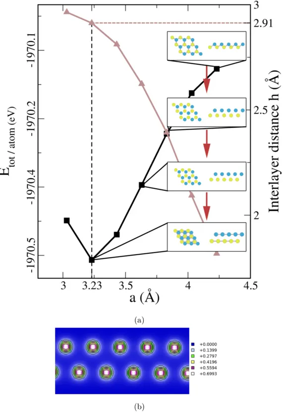
Koristeći analogiju s drugim postojećim dvodimenzionalnim materijalima, pretpostavili smo da će moguće dvodimenzionalne strukture antimona, indija i aluminija poprimiti jedan od četiri oblika. To su ravninska saćasta (Slika 2.1), označena kaoα, svijena saćasta (Slika 2.3), označena kao β, ravninska trokutasta (Slika 2.4), označena kao γ, i naborana (Slika 2.5), označena kao δ. Nakon što su atomi antimona, indija i aluminija stavljeni u pretpostavljene strukture, relaksacijom jedinične ćelije i položaja atoma (Tablica 2.1) dobiveno je da antimon poprimaα,β iδstrukturu, a indij i aluminijα iγ. Zaβ iδ oblike indija i aluminija pokazano je da su dvoslojiγ strukture (Slika 2.8 i Dodatak B), odnosno, da indij i aluminij energetski ne podržavaju dvo-dimenzionalne strukture sastavljene od dva podsloja. Za sve strukture dobiveno je slaganje sa prijašnjim teorijskim rezultatima i eksperimentalnim veličinama, osim u slučaju δ-Sb kod kojega se jedna od konstanti rešetke razlikuje za 4%. U skladu s nazivljem ostalih dvodimenzionalnih materijala, naše strukture nazivamo antimonen, indijen i aluminen.

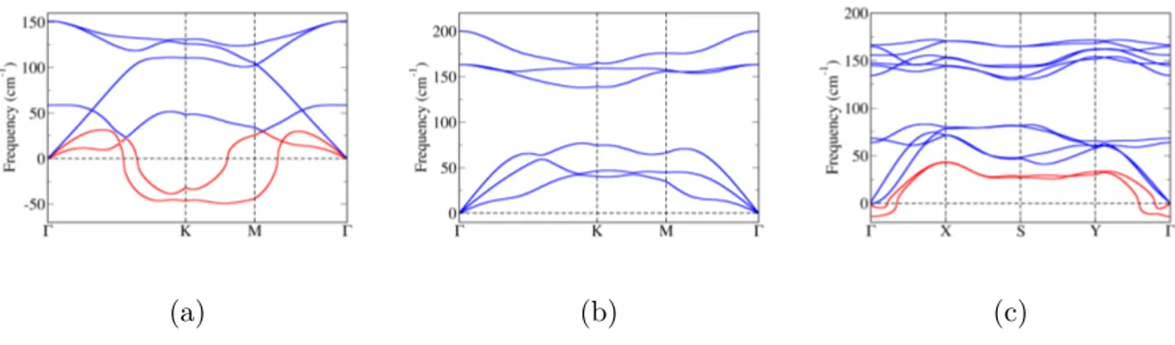
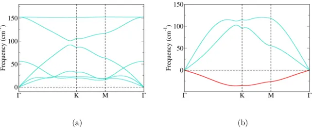
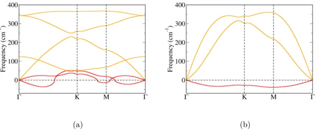
Za dobivene strukture izračunate su fononske disperzije. Realne fononske disperzije nužan su preduvjet stabilnosti kristalne rešetke. Za β-Sb dobivene su realne fononske disperzije, što je u skladu s prijašnjim teorijskim istraživanjima, no kod α-Sb i δ-Sb u određenim smjerovima duž Brillounove zone postoje imaginarne frekvencije (nestabilni fononski modovi). Naši rezultati za δ-Sb nisu u skladu s prijašnjim istraživanjima, no razlike se javljaju zbog ranije spomenute razlike u konstantama rešetke. α-In ima realne fononske disperzije, dok α-Al posjeduje dva nestabilna fononska moda. γ strukture oba elementa imaju nestabilne fononske disperzije.

Deformacija struktura i stabilnost

Deformacija je iznimno jednostavan način za moduliranje svojstava dvodimeninzionalnih materijala te se u eksperimentima može na različite načine nametnuti na

(12)

dvodimenzion-alnu strukturu. Stoga je proučavan utjecaj deformacije na jediničnu ćeliju istraživanih struktura. Bilo koja deformacija u dvodimenzionalnim kristalima može se opisati defor-macijom u armchair i zigzag smjeru. Homogena deformacija u svim smjerovima naziva se biaksijalna deformacija. Koristili smo izravnu deformaciju heksagonalne rešetke (Slika 3.3) što nije bio slučaj u prijašnjim istraživanjima. Ovakav pristup omogućio nam je konzistentnost pri promatranju utjecaja deformacije na slobodnu strukturu, posebno pri računanju fononskih disperzija. Također, velika prednost je manje trajanje simulacija u odnosu na pravokutne jedinične ćelije kakve su korištene u ostalim istraživanjima (nije potrebno povećavati broj atoma u jediničnoj ćeliji). Deformacija je simulirana u koracima od 2% od -20% do +40%. Dobivene su relacije odnosa naprezanja i deformacija (Slika 3.4) iz kojih su iščitane kritične deformacije, εcrit, kao maksimum naprezanja (Tablica 3.1).

Kritične deformacije su nam dale granične vrijednosti deformacije za koju bi se struk-tura mogla vratiti u izvorni, nedeformirani, oblik. Iznosi kritičnih deformacija razlikuju se od pojedinih ranije izračunatih vrijednosti, ali pokazuju anizotropnost i sličnu razinu anizotropije.

Izračunate su, također, i fononske disperzije deformiranih struktura. Deformacija uzrokuje promjenu u međusobnim udaljenostima između atoma unutar jedinične ćelije te time mijenja frekvenciju fonona. Fononske disperzije svih struktura za sažimajuće defor-macije posjeduju imaginarne frekvencije pojedinih modova (Dodatak C). Sve strukture antimonena posjeduju imaginarne fononske frekvencije za bilo koji iznos deformacije, što ukazuje da deformacija kristalne rešetke nije čimbenik koji ju stabilizira, jer sve tri su eksperimentalno ostvarene. Za strukture indijena i aluminena dobivena su područja sta-bilnosti za određene iznose deformacije što ukazuje na mogućnost njihove eksperimentalne sinteze. Rezultati su sažeti na Slici 3.12.

Supstrati

Pošto se deformacija javlja prirodno pri sintezi na supstratima, identificirane su metalne površine i drugi dvodimenzionalni materijali koji mogu poslužiti kao supstrat. Računi su konvergirani za Ag(111), Cu(111) i grafen. PdTe2 kao supstrat je korišten samo u slučaju

α-Sb i β-Sb. Pri postavljanju dvodimenzionalne strukture na supstrat, javlja se a priori

biaksijalna deformacija kristalne rešetke, no pošto se atomi relaksiraju u energetski na-jpovoljnije položaje, ova deformacija može poprimiti armchair ili zigzag karakter (Tablica

(13)

4.1).

Za strukture antimonena dobiveno je ponašanje u skladu s eksperimentalnim rezulta-tima. Na ravnim metalnim površinama, β-Sb prelazi u α-Sb i posjeduje iste parametre rešetke. Obavljen je i pomoćni račun na PdTe2, s neravnom površinom, na kojem α-Sb

prelazi u β-Sb. Ovi rezultati pokazuju da tip i izgled supstrata utječu na strukturu an-timonena koja će se sintetizirati na njegovoj površini. Pri postavljanju β-Sb na grafen, on zadržava svoj β oblik. Postavljanje δ-Sb na ranije spomenute supstrate daje različite oblike dvosloja α-Sb i β-Sb.

Zaα-In i α-Al identificirani su supstrati koji, u skladu s deformacijama koje vrše na njihovu kristalnu rešetku, mogu služiti kao supstrat za njihovu eksperimentalnu sintezu. U α-In slučaju to su Ag(111), Cu(111) i grafen, a uα-Al slučaju to su Cu(111) i grafen. Simulacijama molekularne dinamike dvodimenzionalnih struktura na supstratima ispi-tana je njihova stabilnost na sobnoj temperaturi. One pokazuju termičko gibanje oko ravnotežnih položaja, bez raspadanja struktura na više različitih vremenskih skala, što je i potvrđeno i funkcijama radijalnih distribucija atoma (Slika 4.6).

Karakterizacija

Izračunate su elektronska struktura vrpci (Slike 5.1 i 5.2), optička (Slike 5.3 - 5.7) i elastična svojstva (Tablica 5.1). α-Sb iβ-Sb pokazuju poluvodički karakter s procjepima od 1.31 eV i 0.06 eV. Isključivo p-orbitale pridonose najvišim stanjima valentne vrpce i najnižim stanjima vodljive vrpce. Sve α strukture pokazuju metalni karakter. Rezultati se kvalitativno slažu s prijašnjim istraživanjima. Optička svojstva pokazuju anizotropnost ovisno o polarizaciji upadnog elektromagnetskog značenja, karakterističnu dvodimenzion-alnim materijalima. Optička svojstva α-In i α-Al pokazuju aktivnost u optičkom dijelu spektra, poput većeg postotka refleksije nego slični dvodimenzionalni materijali. Elastična svojstva su slična ostalim dvodimenzionalnim materijalima, uz to da α-Sb pokazuje iz-vanredno visok Poissonov omjer, dok α-In niži nego ostali materijali. Razlike dolaze od različite karakteristike vezanja i jakosti vezanja. U slučaju α-In radi se o vezi kovalentnije prirode i slabije jakosti, dok kod α-Sb veza je više metalnog karaktera (Slika 5.7).

(14)

Zaključak

Rezultati ove disertacije proširili su bazu poznatih dvodimenzionalnih materijala i pred-vidjeli su eksperimentalne uvjete potrebne za njihovu sintezu - vrsta i simetrija korištenog supstrata, potrebna deformacija da bi se ostvarila stabilna dinamika kristalne rešetke i odgovarajuća temperatura na kojoj bi se mogla vršiti sinteza. Korištena je nova metoda deformacije kristalne rešetke kako bi istražili dinamičku stabilnost kristalne rešetke. Ispi-tana su strukturna svojstva i dana je karakterizacija novih potencijalnih dvodimenzion-alnih struktura antimona, indija i aluminija. Za proširenje rezultata ove disertacije, potrebno je istražiti dodatne supstrate radi šireg izbora pri eksperimentalnoj sintezi, a njihove karakteristike bi se trebale ispitati nekima od kompleksnijih aproksimacija teorije funckionala gustoće. Iako rezultati istraživanja daju nadu u eksperimentalnu sintezu ovih materijala, treba spomenuti njihovu tendenciju da oksidiraju u atmosferi. Za njihovu eventualnu primjenu, potrebno je istražiti načine njihove zaštite. Također, proučavanje niskodimenzionalnih oksida ovih elemenata je možda ključan korak u budućem istraži-vanju i njihovoj primjeni.

(15)

Keywords

two-dimensional materials, antimony, indium, aluminium, density functional theory, strain engineering

(16)

Introduction

New science and technology are the driving forces for the progress of human race. This is almost not to be contested, it seems logical enough - we can see the mankind’s progress all around us and the world is much more different than, for example, one hundred years ago - mostly due to the breakthroughs in science and new technologies that follow from it. Since the dawn of the human race, new materials were what gave us the advantage over our competitors and against the force of nature. As a grim example, one could mention the introduction of iron smelting was what gave the figurative and literal edge to new civilizations, or, as newer, more positive example, the new materials for semiconductors that improve IT technology or new materials for solar cells that improve our capabilities of harvesting the almost infinite energy of the Sun.

The requirements of the modern world for new materials for potential applications are lower manufacturing costs, smaller dimensions (the everlasting need for miniaturization) and improved properties. So, the research should be focused to at least improve some of the, if not all the requirements. In the last 15 years, a new field of materials has developed - the field of low-dimensional materials - whose at least one dimension is degrees of magnitude smaller that the others. A subfield of low-dimensional materials are two-dimensional materials, whose third dimension is suppressed and consists of only a few layers or even one layer of atoms. Two-dimensional materials fulfil the first two conditions in a natural way. The smaller dimensions are obvious and lower manufacturing costs also, at least in the amount of raw material needed for their production. The third condition, improved properties, can be accounted for by modifying their structure with state-of-the-art theoretical and experimental procedures, if they do not possess them outright.

Since the first experimental realisation of single sheet of carbon atoms - graphene - two-dimensional materials have been subject to numerous scientific research, both theoretical and experimental. Two-dimensional materials present a door to interesting new physics,

(17)

but also have immense application potential.

Graphene was first obtained by Geim and Novoselov[1] in 2004 from graphite, with a simple method called micromechanical cleavage. Since then, new methods for obtaining graphene were developed, such as chemical vapour deposition (CVD), thermal decom-position of compounds, etc. Mechanical cleavage, however, remains one of the primary methods of obtaining high-quality graphene crystals. Graphene is know for its honeycomb lattice, in which every carbon atom is bound with three others. Since carbon contains four valence electrons, it undergoes sp2 _{hybridization to form strong} _σ_{in-plane bonds}

be-tween them, while out-of-plane they are bound with weakπbonds. Graphene is a zero-gap semiconductor, with valence and conducting bands meeting at the K-point of the Brilloun zone. But, due to its unique linear dispersion around it, forming the so-called Dirac cones, the charge carriers have high velocities, on the order of 106 _{m/s [2]. Experimental}

mea-surements give many excellent properties of graphene, such as room-temperature electron mobility of 2.5×105 _cm2_V−1_s−1_{[3], Young’s modulus of 1 TPa [4] and a very high thermal}

conductivity [5]. However, its zero-gap characteristics are a problem for applications in electronic devices.

Also belonging to the field of high-researched two-dimensional materials are transition metal dichalcogenides (TMDs), whose monolayer consists of a transitional metal atom (Mo, W, Pd etc.) layer sandwiched between two layers of chalcogen atoms (S, Se, Te). These monolayers are direct-gap semiconductors, and they can be used in transistors. Like graphene, they can be obtained by mechanical exfoliation from their bulk form, but they can also be obtained by other, chemical methods. They have direct band gap, strong spin-orbit coupling and applicable electronic and mechanic properties [6].

Due to the same valence configuration as carbon, other Group IV elements can pos-sess allotropes in analogue to carbon. Silicon, germanium and tin two-dimensional al-lotropes, called silicene, germanene and stanene, have been predicted and synthesized[7– 9]. Two-dimensional allotropes of other elements have also been found, like borophene[10], phosphorene[11] and antimonene[12].

Although various two-dimensional allotropes and materials have been predicted and acquired in the experiment, there is still much room for growth, given the still relatively new nature of the field and no material with ideal properties. Hence, there is place for new materials and their potential application. Inside this thesis, we focus on two dimensional

(18)

allotropes of antimony, indium and aluminium.

Two-dimensional antimony allotropes have already been experimentally acquired [13– 16] and there has been research studying its electronic, optical and mechanical properties [17–19]. However, what remains unclear is what governs the antimonene synthesis and the prefered allotrope acquired, which we try to inspect in this thesis. Also, antimonene has showed remarkable stability in air, which promises potential use in every day situations. Although boron two-dimensional allotropes have been found, the experimental real-ization still remains sparse [20]. Other elements of the boron group - aluminium and indium - have not been researched in great detail. Some theoretical studies exist and we will be drawing upon them in the remainder of this thesis, however, no conclusive results have been published on aluminium and indium two-dimensional allotropes. The basic motivation to study these two elements comes from the facts that aluminium is the most abundant metal in the Earth’s crust. It is low cost, has recyclable nature and has lightweight characteristics, while indium is widely used in different alloys, semi-conducting materials and coatings, promising wide potential use of devices based on its two-dimensional allotropes.

The hypothesis of this thesis is that among the so far unconsidered elements of Group IIIA and VA, stable allotropic modifications of monolayer structures can be found. These structures should have elastic, electronic and optical properties which surpass or com-plement the properties of known monolayer materials. The studied materials are to be connected with applications in the electronic and optical industry through the insights into the ability to experimentally synthesize the studied structures. This thesis will ex-pand on the knowledge of known monoelement two-dimensional structures which provides possibilities on their application in novel devices at the nanoscale.

In this thesis, using density functional theory (DFT) we focus on structural properties of antimony, indium and aluminium two-dimensional allotropes, their behaviour under strain and their structure on substrates, as well as their characteristics of identified al-lotropes. Density functional theory has been extensively used as an ab initio theoretical method for prediction of stable two-dimensional structures and verification of experimen-tal results. However, as with any theoretical approach which uses approximations, one should be careful proceeding with results acquired, as they depend on the level of theory and pseudopotentials used.

(19)

Chapter 1 Theoretical background

1.1 Born-Oppenheimer approximation

We are presented with a system of nuclei and electrons in some arrangement. What we would like to do is find the states and energies of the given system. The Hamiltonian is given by ˆ H =− ~ 2 2me X i ∇2 i − 1 4π0 X i,I ZIe2 |ri−RI| + 1 8π0 X i6=j e2 |ri−rj| − ~ 2 2MI X I ∇2 I+ 1 8π0 X I6=J ZIZJe2 |RI−RJ| , (1.1)

where electrones and nuclei are denoted by uncapitalized and capitalized subscripts, re-spectively. The first and the fourth terms are the kinetic energies of electrons and nuclei, respectively, second is the Coulomb interaction between the electrons and the nuclei and the remaining two terms are the Coulomb electron-electron and nuclei-nuclei interaction. The wavefunction of the system is given by the stationary Schrödinger’s equation:

ˆ

Hψ =Eψ , (1.2)

which is, but for the simplest of cases, unsolvable. From here on out, we will be using Hartree atomic units where _~=e=me = 4π0 = 1.

As the mass of the nuclei is orders of magnitude larger than the mass of the electrons, nucleonic motion, from the electron point of view, appears frozen. With that in mind, in (1.1), the kinetic energy of the nuclei,

ˆ TN = 1 2MI X I ∇2_I , (1.3)

(20)

1.1. Born-Oppenheimer approximation

can be considered "small" relative to the other terms, so we can treat it as an perturbation:

ˆ

H = ˆHe,n+ ˆTn . (1.4)

The unperturbed part, ˆHe,n, only depends on RI (the position of the nuclei)

parametri-cally. Ignoring the kinetic nuclear part, hamiltonian for electrons of the starting system is:

ˆ

H = ˆT + ˆVee+ ˆVen+Enn , (1.5)

where ˆT is kinetic energy operator of the electrons ˆ T = 1 2 X i ∇2 i , (1.6) ˆ

Vee is the electron-electron interaction

ˆ Vee= 1 2 X i6=j 1 |ri−rj| , (1.7) ˆ

Venis the electron-nuclei interaction, which in the exact case is the Coulumb interaction,

but also can be expressed as a fixed potential acting on the electrons of the system ˆ

Ven=

X

i,I

VI(|ri−RI|), (1.8)

and Enn is the nuclei-nuclei interaction that only contributes to the total energy of the

system but does not influence our quantum mechanical description of the electrons. For the purpose of finding the solution to (1.2) it can be neglected and added later.

We are left with a form of hamiltonian that is called the electronic hamiltonian: ˆ

He = ˆT + ˆVee+ ˆVen . (1.9)

Its solution gives us the electronic wavefunctions ψe which are functions of electronic

coordinates ri, but are parametrically dependent on the positions of the nuclei RI

-meaning that changing the coordinates of the nuclei changes the form of ψe. Inserting

(1.9) into (1.2) instead of full ˆH

ˆ

Heψe=Eeψe (1.10)

gives us the electronic energy - Ee- in some outer potential ˆVen due to the nuclei. Adding

back the Enn, we acquire the total energy of the system

(21)

1.1. Born-Oppenheimer approximation

for a given set of nuclei positions RI.

Now we go back to the full hamiltonian of the system, (1.1). Looking at electronic motion from the nuclei point of view, it is orders of magnitude greater that nucleonic motion. What nuclei "see" is the average of the electronic motion and it is reasonable to replace all the electronic contributions in (1.1) by their average over the electronic wavefuntion ψe ˆ H =h−1 2 X i ∇2 i − X i,I ZI |ri−RI| +1 2 X i6=j 1 |ri−rj| i − 1 2MI X I ∇2 I+ 1 2 X I6=J ZIZJ |RI−RJ| , (1.12)

which is nothing other that electronic energy Ee and together with the last term (which

produces Enn) ˆ H =− 1 2MI X I ∇2 I+Ee+Enn , (1.13)

we acquire the hamiltonian for the nucleonic motion ˆ H =− 1 2MI X I ∇2 I+Etot(RI), (1.14)

where we have written dependence of the Etot onRI explicitly. (1.14) gives us the motion

of the nuclei in a potential formed by solving the electronic motion. Molecular dynamics

If we treat the problem of nucleonic motion classically, we can write MI ∂2_R I ∂t2 =FI(R) = − ∂ ∂RI E(R). (1.15)

To acquire the motion of nuclei, we can use a numerical solution to the above equation using discrete time steps, such as the Verlet algorithm or any other type numerical solution to a differential equation. Using the Verlet algorithm, positions of nuclei at the next time instance, t+ ∆t (where ∆t is the time step) depend on the forces in the present time step

RI(t+ ∆t) = 2RI(t) +RI(t−∆t) +

(∆t)2

MI

FI{RI(t)}. (1.16)

In the above equation, the second derivative with respect to time was replaced with an approximation

f00(x)≈ f(x+h)−2f(x) +f(x−h)

(22)

1.2. Crystal structure

The correct forces on nuclei are determined by the electronic motion and nucleonic po-sitions, so correct solution to electronic motion is necessary for obtaining the correct nucleonic motion.

What was presented here was qualitative description of finding a solution for a given system of atoms. There are different ways of finding the solution to electronic problem and consequently the full state of the system, but the one that will be used in the scope of this thesis is the density functional theory (DFT).

1.2 Crystal structure

The crystal structure is determined by a primitive cell, together with positions of atoms inside of it, called the basis, and a set of translations that produce the periodicity. The set of all translations forms a lattice in space (Bravais lattice) and any translation can be written as integral multiples of the primitive cell vectors a1,a2, ...

T(n1, n2, ...) = n1a1+n2a2+... . (1.18)

With each lattice there is an associated reciprocal lattice, defined (in 3D) as bi= 2π

aj×ak

|ai(aj×ak)|

, (1.19)

where i, j, k are cyclical permutations of coordinates. Primitive cell in reciprocal space is called the first Brillouin zone. For a crystal that possesses translational symmetry, the Bloch theorem allows for eigenstates of translation operators to differ from one cell to another only by a phase factor

Tψ(r) =eik·Tψ(r), (1.20) wherekis any wavevector inside the Brillouin zone. Applying it to Schrődinger’s equation for a system with a periodic Hamiltonian, like a crystal, we can further use the Bloch theorem to write

ψk(r) =eik·r uk(r), (1.21)

where uk is a periodic function with the same periodicity as the crystal.

For a large enough volume, i.e. macroscopic crystal,kvalues become continuous. The Hamiltonian is defined for each kand by solving it we get discrete eigenstates

(23)

1.2. Crystal structure

with eigenvalues i,k. The eigenvalues i,k form what is called energy bands - with

possi-bility that there exists a range of energies that have no associated states, for any k, called energy gaps.

For certain properties of the crystal, like total energy, a sum over allkstates is needed. For a general function fi(k), where iis a set of discrete states at a certain kthe average

value per cell is

f_i = 1 Nk

X

k

fi(k), (1.23)

where Nk is the number of k values. With Nk going to infinity, the sum becomes an

integral of the form

f_i = 1 ΩBZ

Z

BZ

dkfi(k), (1.24)

where ΩBZ is the volume of the Brillouin zone. In practice we choose a discrete set of

points for the approximation of this integral. A general method proposed by Monkhorst and Pack gives a uniform set of points given by [21]

kn1,n2,n3 = 3 X i 2ni−Ni−1 2Ni bi . (1.25)

A grid defined as above has useful properties, such as being offset from the points k= 0 and, if chosen to be even, omits the high-symmetry points.

1.2.1 Structural optimization

In a periodic crystal, the optimized structure is given by the vectors of the unit cell and positions of the atoms inside it. The equation (1.14) gives us the Hamiltonian for nucleonic motion. By finding the minima of the potential surface we obtain the optimized structure of the system. From the Hellman-Feynman theorem [22], forces on the nuclei can be obtained by

FI =−

∂E ∂RI

, (1.26)

whereE is the total energy andRI are the positions of the nuclei. By finding a

configura-tion where the forces on atoms are zero, we in principle arrive at the optimized structure. Since this is a calculation problem in parameter space of{RI}(3N variables), specialized

algorithms are used for structure optimizations. In this thesis, we have used the BFGS algorithm developed by Broyden, Fletcher, Goldfarb and Shanno [23] implemented inside the used computer code.

(24)

1.3. Density functional theory (DFT)

1.3 Density functional theory (DFT)

The usual method of dealing with quantum mechanical problems is solving the Schröd-inger’s equation for some potential ˆV and acquiring wavefunctions ψn of the system as

the eigenfunctions of the hamiltonian. If our problem dealt with a system of electrons, for example like in (1.9), hamiltonian depends on electron coordinates, ri, the number of

which is 3N, where N is the number of electrons. From that set of eigenfunctions, the one with the lowest energy is the ground state ψ0(ri) and using it, we can find different

properties of the system, including the ground state density n0(r).

What density functional theory proposes is solving the problem in terms of electron density n(r), and reducing the number of variables from 3N to only 3.

1.3.1 The Hohenberg-Kohn theorems

The Honenberg-Kohn theorems deal with many-body interacting systems, such as the one from 1.9. We can write hamiltonian of such a system in general as

ˆ H =−1 2 X i ∇2 i − X i Vext(ri) + 1 2 X i6=j 1 |ri−rj| , (1.27)

where Vext is some kind of external potential acting on the electrons of the system.

The-orems are stated as follows[24]:

Theorem I - For any system of interacting particles in an external potential Vext(r),

the Vext(r) is determined uniquely, except for a constant, by the ground state particle

density n0(r).

Theorem II - A universal functional for the energy E[n] in terms of the density n(r)

can be defined, valid for any external potential Vext(r). For any particular Vext(r), the

exact ground state energy of the system is the global minimum value of this functional, and the densityn(r) that minimizes the functional is the exact ground state densityn0(r).

The proof to both is simple and can be found in original paper by Honenberg and Kohn [25]. What follows from the theorems is that since the ground state density n0(r)

(25)

and from hamiltonian all of the wavefunctions follow, meaning that ground state density n0(r) also determines all the properties of the system. Also, the functionalE[n] is enough

to determine the ground state density n0(r) of the system. The total energy functional is

given by

E[n] =T[n] +Eint[n] +

Z

d3r Vext(r)n(r) +Enn (1.28)

and finding it’s minimum in respect to density n(r) gives us the ground state density n0(r).

1.3.2 Kohn-Sham approach

In principle, (1.28) gives us a way to find the ground state density n0(r) of the system.

What it does not answer is how we extract any meaningful information from it - like we could from the wavefunction of the system. Also, multi-body interacting systems are difficult to solve. To deal with this problem, we assume that there exists a non-interacting system of particles with the same ground state density n0(r) as the starting

system - finding solution to such a system gives us the properties of the fully interacting system because they share the same ground state density n0(r).

The energy functional (1.28) is rewritten as EKS =− 1 2 X i hψi|∇2|ψii+ 1 2 Z d3rd3r0n(r)n(r 0₎ |r−r0_| + Z d3rVext(r)n(r)+Enn+Exc[n], (1.29) with n(r) = X i |ψi(r)|2 , (1.30)

where ψi are the wavefunctions of the non-interacting electrons.

In (1.29) the first term is the kinetic energy of non-interacting electronsTs[n], second

term is the Coulumb interaction of the density with itself (called Hartree energy). The third term is the energy of electrons in the potential of the nuclei and the fourth is the energy of the nuclei-nuclei interaction. The fifth term is called the exchange-correlation energy, incorporating both Hartree-Fock exchange of electrons with the same spin, as well as correlated motion of electrons due to Pauli exclusion principle[26]. Finding the minimum of the new energy functional brings us to Schrődinger-like set of equations for ψi called Kohn-Sham[27] equations:

(26)

where HKS is the effective hamiltonian of the electrons

HKS =−

1 2∇

2₊_V

ext(r) +VHartree(r) +Vxc(r). (1.32)

All the terms in (1.32) are well defined except the final - Vxc(r) - and quality of our

solution to Kohn-Sham equations will depend on the right description or approximation of the exchange-correlation effects.

1.3.3 Approximations for the exchange-correlation functional

Local-density approximation (LDA)

We get the simplest form for exchange-correlation effects by making an assumption that it only depends on the density at a certain point (local density). Writing

E_xcLDA[n] = Z

d3r xc(n)n(r), (1.33)

where xcis the exchange-correlation energy per particle, we get the exchange-correlation

energy depending only on the form of xc. The local dependence can be written in many

ways, but for LDA it is usually taken as the exchange-correlation energy per particle of homogeneous electron gas - HEG

xc - which can be separated into independent terms for

exchange and correlation:

HEG_xc =e+c. (1.34)

Exchange energy per particle for homogeneous electron gas is know explicitly, and given with x =− 3 4π _9π 4 1/3 r_s−1 , (1.35)

wherers is parameter describing the density of the system, given as a radius of the sphere

containing a single electron

4π 3 r 3 s = 1 n . (1.36)

Correlation energy can only be given approximately [Ref]. Generalized gradient approximations - GGA

Further step in improving our approximation is including the dependence of the exchange-correlation energy on the changes in the density at a certain point - it’s gradient:

E_xcGGA[n] = Z

(27)

with

xc =HEGx Fxc, (1.38)

where Fxc is dimensionless function of the density gradient. The form of this function

is not given exactly and depends on the type of the generalized gradient approximation used, like PW91[28] or PBE[29].

Further improvements of XC approximations

For materials with localized and strongly interacting electrons, often an additional orbital-dependant interaction term is introduced, with the form same as the Hubbard model [30]. Such approach is called "DFT+U" and it improves on the the results of LDA and GGA calculations (such as the band gap of materials) of strongly correlated systems such as transition metal oxides.

Although not used in the research present in this thesis, there are further ways to enhance the exchange-correlation energy functional. The next "logical step" could be including dependence on higher gradients of density, going by the name of meta-GGA. Also, combining DFT expression for the exchange-correlation with a term calculated using Hartree-Fock theory produces the so-called "hybrid functionals", with the mixing of different contributions depending on the type of functional used [31].

1.3.4 Solving Kohn-Sham equations

Now we approach the solving of Kohn-Sham equations −1 2∇ 2₊_V ef f(r) ψi(r) =iψi(r) (1.39) with Vef f(r) = Vext(r) +VHartree(r) +Vxc(r) (1.40)

being the effective potential acting on the electrons. Assuming we chooseVxc(r), we start

by making an initial guess of the density of the system n(r). We calculate the effective potential in the system, (1.40) and use it to solve the set of Kohn-Sham equations (1.39). Once ψi are calculated, we calculate the electron density

n(r) =X

i

(28)

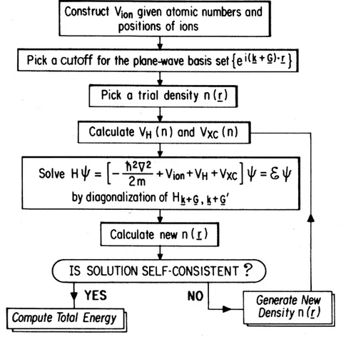
and then check the self-consistency, i.e. test if the density differs from the initial guess (to a chosen degree of precision). If the solution is not self-consistent, we take the output density as our new initial guess and repeat the calculation. The loop is done until the self-consistency is reached. Once we find a self-consistent solution, one can proceed to calculating physical quantities of the system. The algorithm is shown in Fig. 1.1.

Figure 1.1: Algorithm for iterative self-consistent solution to Kohn-Sham equations. Taken from reference [32].

Plane wave basis

If we perform a Fourier transform of ui,k(r) from 1.22, we get

ui,k(r) =

X

m

ci,m eiGm·r, (1.42)

where Gm are wavevectors in reciprocal space with integer number peridocity of the

crystal. Inserting it back to 1.22, we get ψi,k(r) =

X

m

(29)

In principle, the sum in above equation is infinite, but for all practical purposes a cut-off energy is chosen, such that the expansion in (1.43) satisfies some chosen degree of precision.

1.3.5 Pseudopotentials

Broadly speaking, we can separate electrons in atoms into two categories - tightly bounded inner electrons ("core") and outer, more loosely bounded electrons ("valence"). In general, bonding of molecules or solids is done through the interactions between valence electrons. Also, the true valence wavefunctions are extremely oscillatory near the core (having a large amount of nodes), to ensure the orthogonality with core wavefunctions. To ensure accurate enough expansion of wavefunctions, a lot of plane waves have to be included in the basis (1.43), increasing the complexity of calculation.

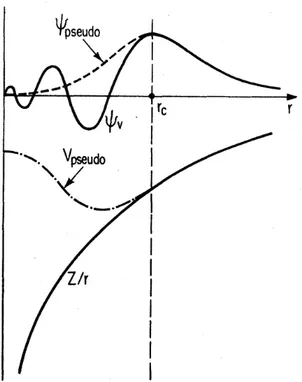
Figure 1.2: Illustration of an all-electron wavefunction and potential (solid lines) and pseudowavefunction and pseudopotential (dashed lines). Radius beyond which they match is designated with rc. Taken from reference [32].

The aim of pseudopotentials is to simplify the electronic problem by dealing with both issues - by only including the valence electrons and replacing their Coulomb interaction

(30)

with the nucleus and inner electrons with an effective potential (the frozen core approx-imation) while also "smoothing out" their form near the core. Pseudopotentials replace the all-electron wavefunctions with pseudo-wavefunctions which match beyond some core cutoff radiusrc to ensure right kind of behaviour in the space between atoms where most

of bonding and physical properties take shape, while differing inside where the exact physical description is not necessary (Fig. 1.2).

Details on the types of pseudopotentials used in our calculations are shown in Ap-pendix A.

Norm-conserving pseudopotentials

Norm-conserving pseudopotentials are characterized by the norm-conserving condition which demands that both the radial all-electron wavefunction and pseudo-wavefunction integrate to the same amount of charge in the chosen core radius rc

Q= Z rc 0 dr r2|ψ(r)|2 ₌Z rc 0 dr r2|ψP S(r)|2 _. _(1.44)

Beyond the cutoff radius rc all-electron and pseudo valence wavefunctions have to match,

with their eigenvalues also being the same. Also, the logarithmic derivatives of all-electron and pseudo wavefunctions have to agree at rc.

Ultrasoft pseudopotentials

Ultrasoft pseudopotentials relax the norm-conserving condition (1.44) by adding auxiliary functions around ion cores which take into account the oscillatory character of all-electron wavefunctions. This allows for increased smoothness of the pseudowavefunctions, reducing the complexity of calculation, but increasing the accuracy to some extent.

1.3.6 Ab initio molecular dynamics

Within the Born-Oppenheimer approximation, also called the adiabatic approximation, the electrons stay in their instantaneous ground state as the nuclei move. The total energy of the system of electrons and nuclei, within the Kohn-Sham approach is

E[{ψi},{RI}] = 2 N X i=1 Z ψ∗_i(r) −1 2∇ 2_ψ i(r)dr+Ee[n] +Enn[{RI}], (1.45)

(31)

1.4. Density functional perturbation theory (DFPT) where Ee[n] = 1 2 Z drdr0n(r)n(r 0₎ |r−r0_| + Z drVext(r)n(r) +Exc[n]. (1.46)

The forces on the nuclei are then obtained using the by Hellman-Feynman theorem, here repeated as

FI =−

∂E ∂RI

. (1.47)

When forces on nuclei are know, the molecular dynamics (movement of nuclei) are solved with (1.16) or a similar method for solving differential equations. We have used exactly Verlet algorithm for nucleonic motion.

1.4 Density functional perturbation theory (DFPT)

1.4.1 Response function

If the strength of some small perturbation to the hamiltonian is described by the parameter λ, we can expand the energy, potential or the wavefunctions of the system in term ofλ, i.e. E =E(0)+λE(1)+λ2E(2)+... , (1.48) where E(n) = 1 k! dk_E dλk . (1.49)

The first order corrections to the wavefunctions of the system are given by ∆Ψi = X j6=i Ψj hΨj|∆ ˆH|Ψii Ei−Ej . (1.50)

In the perturbation theory, a "2n+1" theorem is used, which states that if the wavefunction is determined to all orders from 0 to n, the energy of the system to order 2n + 1 is determined. Applying the perturbation theory to density functional theory, we can write for the first order perturbation

∂E ∂λi = ∂Enn ∂λi + Z ∂V ext(r) ∂λi n(r)dr (1.51)

and for the second order perturbation ∂2_E ∂λi∂λj = ∂ 2_E nn ∂λi∂λj + Z ∂2V ext(r) ∂λi∂λj n(r)dr+ Z n(r) ∂λi ∂Vext(r) ∂λi dr. (1.52)

(32)

1.4. Density functional perturbation theory (DFPT)

What we get is the response of the energy to the perturbation in the second order per-turbation theory. The problematic term is the ∂n(r)/∂λi, representing the change of the

density with respect to the perturbation (to the first order). This is equivalent to knowing the first order change of the wavefunctions to obtain the second order correction to the energy. Using the chain rule, we can write the problematic third term in (1.52) as

Z ∂V ext(r0) ∂λi ∂n(r) ∂Vext(r0) ∂Vext(r) ∂λj drdr0 = Z ∂V ext(r0) ∂λi χ(r,r0)∂Vext(r) ∂λj drdr0 , (1.53) where χ(r,r0) is the density response function. χ(r,r0) can be found using the relation

χ=χ0[1 +Kχ], (1.54)

where χ0 _{is the response function, defined as}

χ0_n(r,r0) = δn(r) δVef f(r0 = 2 occ X i=1 empty X j ψ∗_i(r)ψj(r)ψ∗j(r 0_)ψ i(r0) i−j , (1.55)

and K is the kernel defined as

K(r,r0) = 1 r−r0 −

δ2_E

xc[n]

δn(r)δn(r0₎ , (1.56)

which incorporates the Coulomb interaction and the exchange-correlation effects. χ can also be found by using its relation with the inverse dielectric function

−1 = 1 + χ

|r−r0_| . (1.57)

Although the answer to the perturbation is given by finding the right form for the density response function χ, the correct form is difficult to obtain except in the simplest of cases, such as homogeneous electron gas. The response function χ0 and the inverse dielectric function −1 are calculated using unoccupied states the system, of which there could be an infinite number. In principle, we would sum over enough unoccupied states until arbitrary convergence threshold is reached, which is often a problematic task.

1.4.2 DFPT

A simpler solution is given by applying the formalism of the perturbation theory to the Kohn-Sham equations directly. The first order change in density is given by

∆n(r) = 2 Re

N

X

i=1

(33)

First order changes to the wavefunctions are given by

(HKS −i)|∆ψii=−(∆VKS −∆i|ψii, (1.59)

where ∆i =hψi|∆VKS|ψii and

∆VKS(r) = ∆Vext(r) +

Z

d(r0)K(r,r0)∆n(r) (1.60) withK(r,r0) defined in (1.56). This approach simplifies the problem of finding corrections to the wavefunctions, given in (1.59), by taking into account that only the unoccupied states contribute to the first-order corrections while the contributions from occupied states cancel out in pairs. By projecting the right-hand side of (1.59) to the unoccupied states, we get (HKS−i)|∆ψii=−Pˆunocc(∆VKS|ψii, (1.61) where ˆ Punocc = 1−Pˆocc = 1− N X i=1 |ψiihψi|. (1.62)

By solving the above equation for the corrections, with ∆VKS given in terms of ∆n(r),

which are itself given by ∆ψi, we get a self-consistent method of finding the

perturba-tion on the system. Unlike the general approach of the response funcperturba-tion, which gives the answer to all possible perturbations, application of DFPT depends on the type of perturbation.

1.4.3 Phonons

Expanding the energy of the system (1.15) in powers of displacements, the first order derivatives are nothing else than equilibrium condition of the nuclei, i.e. the set of equa-tions (1.47) equal to zero, and the higher derivatives describe the zero-point, thermal or perturbed motion of the nuclei

CI,α;J,β = ∂2_E(_R₎ ∂RI,α ∂RJ,β , CI,α;J,β;K,γ = ∂3_E(_R₎ ∂RI,α∂RJ,β ∂RK,γ , ... , (1.63) where C’s are the quantities called force constants, and α, β, ...are cartesian coordinates. Using the harmonic approximation, vibrational modes of frequency ω are given by

(34)

Inserting the above equation into 1.15 we get an equation

−ω2MIuIα =−

X

J,β

CI,α;J,β uJ β , (1.65)

whose solution is given by setting the determinant of the system to zero det 1 √ MIMJ CI,α;J,β−ω2 = 0. (1.66)

In a crystal structure, where atomic displacement eigenvectors also obey the Bloch the-orem, the above equation decouples for different k with frequencies ωi,k, where i =

1, ...,3Nn: det 1 √ MsMs0 Cs,α;s0_,α0−ω_i,2_k = 0. (1.67)

These atomic oscillations in a lattice are called phonons. The set of all ωk for a given i

is called a phonon mode, of which 3 behave as ω → 0 as k → 0 and are called acoustic modes, while the rest are called optic modes. As ωi,k are frequencies of oscillation they

have to be real. If somehow one acquires imaginary frequencies, this result is non-physical and could indicate instability in the lattice dynamics.

Applying the DFPT for finding the phonon dispersions of a crystal, one would calculate the energy of the system under the perturbation, in this case a phonon of wavevector k and then expand the energy in the second order:

E =E0+ 1 2 X I,α X J,β CI,α;J,β uI,αuJ,β , (1.68)

whereCI,α;J,β are the force constants defined in (1.63) anduI,α, uJ,β are the displacements

of the atoms. First order of the expansion is ignored, as it is zero in the energy minimum. Force on a particular atom is then

FI,α =−

X

J,β

CI,α;J,β uJ,β (1.69)

and the Fourier transform of CI,α;J,β, the dynamical matrix DI,α;J,β, gives us the phonon

dispersions by finding it’s eigenvalues for a particular wavevector k and phonon mode i X

J,β

DI,α;J,β i,k=ω2i,ki,k . (1.70)

1.4.4 Elastic properties

The stress tensor σαβ for a particular structure is given by

σαβ =− 1 Ω ∂Etot ∂ uαβ , (1.71)

(35)

1.5. Dielectric function

where uαβ is the strain tensor defined as

uαβ = 1 2 ∂uα ∂rβ + ∂uβ ∂rα ! , (1.72)

with u’s being the displacements. Elastic properties are described by stress strain rela-tions, with elastic constant, to linear order, given as

Cαβ;γδ = 1 Ω ∂2_E tot ∂ uαβuγδ =−∂σαβ ∂ uγδ . (1.73)

For a two-dimensional structure of square, rectangular or hexagonal symmetry, non-zero elastic constants are C11, C22, C12, C66[33], where 1,2,6 are shorter notations for double

indices xx, yyand xy, respectively. Hexagonal structures also have an additional relation which gives C66 as

C66 =

1

2(C11−C12). (1.74)

The in-plane stiffness (2D Young’s moduli) in [10] and [01] directions[33] are given by Y[10] = C11C22−C122 C22 , Y[01] = C11C22−C122 C11 , (1.75)

with Poisson’s ratios

ν[10] = C12 C22 , ν[01]= C12 C11 (1.76) which for hexagonal structures simplify to

Y =C11(1−ν2), ν =

C12

C11

(1.77) as C11 =C22.

Treatment of strain in DFPT is given, in great detail, by Hamman, Wu, Rabe and Vanderbilt in [34]. Strain is treated as a perturbation only trough the metric tensor, and as such the elastic properties can be acquired trough DFPT with the same treatment as other types of perturbation.

1.5 Dielectric function

The imaginary part of the complex dielectric function 2_α,β(ω), when treated within the adiabatic perturbation theory, can be viewed as a response function

2_α,β(ω) = 1 + 4πe 2 ωm2 X n,n0 X k ˆ Mα,β (Ek,n0 −E_k,n)2 ... ... ( f(Ek,n) Ek,n0 −E_k,n+_~ω+i_~Γ + f(Ek,n) Ek,n0 −E_k,n−_~ω−i_~Γ ) , (1.78)

(36)

1.6. Computer codes

where Γ is the adiabatic parameter, Ek,n are the energy eigenvalues,f(Ek,n) is the Fermi

distribution indicating the occupation of bands and ˆMα,β are the matrix elements

ˆ

Mα,β =huk,n0|pˆ_α|u_k,nihu_k,n|pˆ_β|u_k,n0i, (1.79) with n and n0 being occupied and unoccupied bands respectively. uk,n0 are the periodic parts of the Bloch wavefunctions which are further expanded in a plane wave basis set. The real part of the dielectric function can be obtained through Kramers-Kroning relations:

1_α,β(ω) = 1 + 2 π Z ∞ 0 ω02 α,β(ω 0₎ ω02₋_ω2 dω 0 (1.80) Dielectric function defined as in (1.78) does not take into account the non-local contri-butions to the Hamiltonian, meaning that the kernel K used in derivation of a response function (1.56) has the exchange-correlation energy set to zero. This is called the "random phase approximation". Once the dielectric tensor is obtained, one can proceed to calculate the various optical spectra[35], like the absorption spectrum

α(ω) = √2ωq|(ω)| −1_(ω)_, _(1.81) refractive index n(ω) = s |(ω)|+1_(ω) 2 , (1.82) extinction coefficient k(ω) = s |(ω)| −1_(ω) 2 , (1.83) reflection spectrum R(ω) = [n(ω)−1] 2₊_k2_(ω) [n(ω) + 1]2₊_k2_(ω) (1.84)

and energy loss spectrum

L(ω) =

2_(ω)

(1_(ω))2_{+ (}2_(ω))2 . (1.85)

1.6 Computer codes

Throughout this thesis, we have used the theoretical framework of density functional theory implemented inside two software packages. A major feature of both is that they are Open-Source and free to use software.

(37)

1.6. Computer codes

1.6.1 Quantum ESPRESSO

Quantum ESPRESSO[36] is an integrated suite of Open-Source computer codes for electronic-structure calculations and materials modeling at the nanoscale, based on density func-tional theory, pseudopotentials and plane waves. It is an open collaboration, available to everyone, coordinated by the Quantum ESPRESSO Foundation. It includes a set of com-ponents, each designed for a different part of density functional theory. Some capabilities of Quantum ESPRESSO include the ground-state calculations, structural optimization and molecular dynamics, response properties by the DFPT and more. On their official web pages, a database of pseudopotentials that were used in published scientific work is readily available for download. Majority of work carried out in this thesis was done in Quantum ESPRESSO.

1.6.2 ABINIT

ABINIT[37] is a software package whose main code allows, using DFT, calculations of total energy, charge density and electronic structure system composed from electrons and nuclei. ABINIT uses pseudopotentials or projector augmented wave (PAW) atomic data and planewave basis. Using DFPT, ABINIT can calculate the response functions such as phonons, effective charges and similar. ABINIT is distributed under the GNU General Public License.

(38)

Chapter 2 Two-dimensional crystal structures

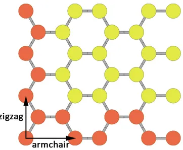
We have chosen the planar honeycomb, buckled honeycomb, planar triangular and puck-ered structures in analogy with other monoelemental two-dimensional materials, as we expect possible structures of proposed elements will the other elements due to similar valence electron structure. Graphene[38], borophene[10], silicine[7], germanene[9] and phosphorene[39] are materials we base our possible structures of antimony, indium and aluminium on.

2.1 Description of crystal lattices

2.1.1 Planar honeycomb

Planar honeycomb structure is chosen in analogue to graphene. Planar honeycomb crystal structure is of hexagonal symmetry (R3m), with Bravais lattice containing two atoms in a lattice basis. Throughout this thesis, we will use shorthandαto refer to planar honeycomb structure. We can choose the unit cell vectors as

a1 =a(1,0,0) a2 =a − 1 2, √ 3 2 ,0 ! a3 =c(0,0,1), (2.1)

where a is the lattice constant (Fig. 2.1) and cis the height of the unit cell. Height c is necessary for the definition of the simulation unit cell, despite the two-dimensional nature of the planar structure. In practice, it is chosen to be large enough to act as a vacuum

(39)

2.1. Description of crystal lattices

above the plane where atoms are placed, and eliminate the interaction between periodic images of the crystal. Each atom has three equidistant neighbours, with distance given by d = a/√3. The angle between bonds is 120◦_{. The unit cell used in computations is}

shown in Fig. 2.1 as the shaded rhombus. The chosen reduced coordinates of the atoms in the cell are

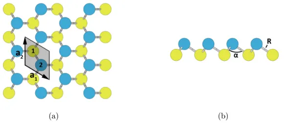
Atom 1 : ₁ 3, 2 3,0 Atom 2 : ₂ 3, 1 3,0 . (2.2) (a) (b)

Figure 2.1: (a) top and (b) side view of α-structure, with in-plane unit cell vectorsa1 and

a2, and bond angle α. Unit cell is shaded gray. Numbers denote atomic positions from

2.2.

The reciprocal lattice vectors are given by

b1 = 2π a 1, 1 √ 3,0 ! b2 = 2π a − 1 2, 2 √ 3,0 ! b3 = 2π c (0,0,1) . (2.3)

(40)

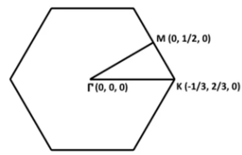
Figure 2.2: The first Brillouin zone of hexagonal unit cell and its high symmetry points.

2.1.2 Buckled honeycomb

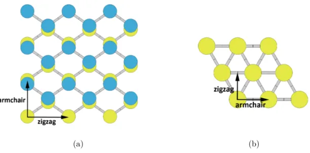
Buckled honeycomb structure is chosen in analogue to silicene and germanene. Buckled honeycomb crystal structure is of hexagonal symmetry (R3m), with Bravais lattice con-taining two atoms in a basis. Throughout this thesis, we will use shorthand β to refer to buckled honeycomb structure.We can choose the unit cell vectors again as

a1 =a(1,0,0) a2 =a − 1 2, √ 3 2 ,0 ! a3 =c(0,0,1), (2.4)

where a is the lattice constant (Fig. 2.3) and c is the height of the simulation unit cell. In the buckled structure, one atom in the basis is found at height h above the lattice plane, also called interlayer distance, thus creating two triangular sublattices. Each atom has three equidistant neighbours with the same angle between bond α. The unit cell used in computations is shown in Fig. 2.3 as the shaded rhombus. The chosen reduced coordinates of the atoms in the cell are

Atom 1 : ₁ 3, 2 3,0 Atom 2 : 2 3, 1 3, h c ! . (2.5)

(41)

(a) (b)

Figure 2.3: (a) top and (b) side view of β-structure, with in-plane unit cell vectors a1

and a2. Two sublattices are designated with different colors. Bottom sublattice atoms are

coloured yellow, while top sublattice atoms are coloured blue. Bond length is designated as R and the angle between bonds is designated as α. Unit cell is shaded gray. Numbers denote atom positions from 2.5.

b1 = 2π a 1, 1 √ 3,0 ! b2 = 2π a − 1 2, 2 √ 3,0 ! b3 = 2π c (0,0,1) . (2.6)

The first Brillouin zone with its in-plane high symmetry points is shown in Fig. 2.2.

2.1.3 Planar triangular

Planar triangular structure is chosen in analogue to borophene. Planar triangular crystal structure is of hexagonal symmetry (R3m), with Bravais lattice containing one atom in a basis. Throughout this thesis, we will use shorthand γ to refer to planar triangular structure. We can choose the unit cell vectors in the same manner as for the honeycomb structure a1 =a(1,0,0) a2 =a − 1 2, √ 3 2 ,0 ! a3 =c(0,0,1), (2.7)

(42)

where a is the lattice constant (Fig. 2.4), and heightc is used in the same manner as in the case ofα-structure. Each atom has six equidistant neighbours with the distance given by d= a. The angle between bonds is 60◦_{. The unit cell used in computations is shown}

in Fig. 2.4 as the shaded rhombus. The chosen reduced coordinates of the atom in the cell is Atom 1 : ₁ 2, 1 2,0 (2.8)

Figure 2.4: Top view of γ-structure, with in-plane unit cell vectors a1 and a2, and bond

angle α. Unit cell is shaded gray. Numbers denote atom positions from 2.8.

b1 = 2π a 1, 1 √ 3,0 ! b2 = 2π a − 1 2, 2 √ 3,0 ! b3 = 2π c (0,0,1) . (2.9)

The first Brillouin zone with its in-plane high symmetry points is shown in the Fig. 2.2.

2.1.4 Puckered

Puckered structure is chosen in analogue to phosphorene. Puckered structure is of or-thorhombic symmetry (Cmca), with Bravais lattice containing four atoms in a basis. Throughout this thesis, we will use shorthand δ to refer to puckered structure. Unit cell

Predviđanje i karakterizacija nisko-dimenzionalnih struktura elemenata antimona, indija i aluminija

Prediction and characterisation of

low-dimensional structures of

antimony, indium and aluminium

Prediction and characterisation of

low-dimensional structures of

antimony, indium and aluminium

Predviđanje i karakterizacija

nisko-dimenzionalnih struktura

elemenata antimona, indija i aluminija

Supervisors’ curriculum vitae

Contents

Acknowledgements

Summary

Sažetak

Keywords

Introduction

Chapter 1

Theoretical background

1.1

Born-Oppenheimer approximation

1.2

Crystal structure

1.2.1

Structural optimization

1.3

Density functional theory (DFT)

1.3.1

The Hohenberg-Kohn theorems

1.3.2

Kohn-Sham approach

1.3.3

Approximations for the exchange-correlation functional

1.3.4

Solving Kohn-Sham equations

1.3.5

Pseudopotentials

1.3.6

Ab initio molecular dynamics

1.4

Density functional perturbation theory (DFPT)

1.4.1

Response function

1.4.2

DFPT

1.4.3

Phonons

1.4.4

Elastic properties

1.5

Dielectric function

1.6

Computer codes

1.6.1

Quantum ESPRESSO

1.6.2

ABINIT

Chapter 2

Two-dimensional crystal structures

2.1

Description of crystal lattices

2.1.1

Planar honeycomb

2.1.2

Buckled honeycomb

2.1.3

Planar triangular

2.1.4

Puckered