El e c t ro n ic
Jo ur
n a l o
f P
r o
b a b il i t y
Vol. 14 (2009), Paper no. 43, pages 1222–1267. Journal URL
http://www.math.washington.edu/~ejpecp/
Random networks with sublinear preferential attachment:
Degree evolutions
Steffen Dereich
∗Institut für Mathematik, MA 7-5, Fakultät II Technische Universität Berlin Straße des 17. Juni 136, 10623 Berlin
Germany
Peter Mörters
†Department of Mathematical Sciences University of Bath
Claverton Down Bath BA2 7AY, United Kingdom
Abstract
We define a dynamic model of random networks, where new vertices are connected to old ones with a probability proportional to a sublinear function of their degree. We first give a strong limit law for the empirical degree distribution, and then have a closer look at the temporal evolution of the degrees of individual vertices, which we describe in terms of large and moderate deviation principles. Using these results, we expose an interesting phase transition: in cases ofstrong
preference of large degrees, eventually a single vertex emerges forever as vertex of maximal degree, whereas in cases ofweakpreference, the vertex of maximal degree is changing infinitely often. Loosely speaking, the transition between the two phases occurs in the case when a new edge is attached to an existing vertex with a probability proportional to the root of its current degree.
Key words:Barabási-Albert model, sublinear preferential attachment, dynamic random graphs, maximal degree, degree distribution, large deviation principle, moderate deviation principle. AMS 2000 Subject Classification:Primary 05C80; Secondary: 60C05, 90B15.
Submitted to EJP on July 30, 2008, final version accepted May 6, 2009. ∗Supported by a grant fromDeutsche Forschungsgemeinschaft (DFG).
1
Introduction
1.1
Motivation
Dynamic random graph models, in which new vertices prefer to be attached to vertices with higher degree in the existing graph, have proved to be immensely popular in the scientific literature re-cently. The two main reasons for this popularity are, on the one hand, that these models can be easily defined and modified, and can therefore be calibrated to serve as models for social networks, collaboration and interaction graphs, or the web graph. On the other hand, if the attachment prob-ability is approximately proportional to the degree of a vertex, the dynamics of the model can offer a credible explanation for the occurrence of power law degree distributions in large networks.
The philosophy behind these preferential attachment models is that growing networks are built by adding nodes successively. Whenever a new node is added it is linked by edges to one or more existing nodes with a probability proportional to a function f of their degree. This functionf, called
attachment rule, or sometimesweight function, determines the qualitative features of the dynamic network.
The heuristic characterisation does not amount to a full definition of the model, and some clarifi-cations have to be made, but it is generally believed that none of these crucially influence the long time behaviour of the model.
It is easy to see that in the general framework there arethreemain regimes:
• thelinearregime, where f(k)≍k;
• thesuperlinearregime, where f(k)≫k;
• thesublinearregime, where f(k)≪k.
The linear regime has received most attention, and a major case has been introduced in the much-cited paper Barabási and Albert[1999]. There is by now a substantial body of rigorous mathematical work on this case. In particular, it is shown in Bollobás et al.[2001], Móri[2002]that the empirical degree distribution follows an asymptotic power law and in Móri[2005]that the maximal degree of the network is growing polynomially of the same order as the degree of the first node.
In the superlinear regime the behaviour is more extreme. In Oliveira and Spencer [2005] it is shown that a dominant vertex emerges, which attracts a positive proportion of all future edges. Asymptotically, afternsteps, this vertex has degree of ordern, while the degrees of all other vertices are bounded. In the most extreme cases eventually all vertices attach to the dominant vertex.
Specifically, we discuss a preferential attachment model where new nodes connect to a random number of old nodes, which in fact is quite desirable from the modelling point of view. More precisely, the node added in thenth step is connected independently to any old one with probability
f(k)/n, where k is the (in-)degree of the old node. We first determine the asymptotic degree distribution, see Theorem 1.1, and find a result which is in line with that of Rudas et al.[2007]. The result implies in particular that, if f(k) = (k+1)α for 0 ¶ α <1, then the asymptotic degree distribution(µk)satisfies
logµk∼ −1−1αk1−α,
showing that power law behaviour is limited to the linear regime. Under the assumption that the strength of the attachment preference is sufficiently weak, we give very fine results about the prob-ability that the degree of a fixed vertex follows a given increasing function, see Theorem 1.13 and Theorem 1.15. These large and moderate deviation results, besides being of independent interest, play an important role in the proof of our main result. This result describes an interesting dichotomy about the behaviour of the vertex of maximal degree, see Theorem 1.5:
• The strong preference case: If Pn1/f(n)2 < ∞, then there exists a single dominant vertex –called persistent hub– which has maximal degree for all but finitely many times. However, only in the linear regime the number of new vertices connecting to the dominant vertex is growing polynomially in time.
• The weak preference case:IfPn1/f(n)2=∞, then there is almost surelynopersistent hub. In particular, the index, or time of birth, of the current vertex of maximal degree is a function of time diverging to infinity in probability. In Theorem 1.8 we provide asymptotic results for the index and degree of this vertex, as time goes to infinity.
A rigorous definition of the model is given in Section 1.2, and precise statements of the principal results follow in Section 1.3. In Section 1.4 we state fine results on the evolution of degrees, which are useful in the proofs of our main results, but also of independent interest. These include laws of large numbers, a central limit theorem and large deviation principles for the degree evolutions. At the end of that section, we also give a short overview over the further parts of this paper.
1.2
Definition of the model
We now explain how precisely we define our preferential attachment model given a monotonically increasingattachment rule f :N∪ {0} −→(0,∞)with f(n) ¶ n+1 for alln∈N∪ {0}. At time
n=1 the network consists of a single vertex (labeled 1) without edges and for eachn∈Nthe graph evolves in the time stepn→n+1 according to the following rule
• add a new vertex (labeledn+1) and
• insert for each old vertexma directed edgen+1→mwith probability
f(indegree ofmat timen)
The new edges are inserted independently for each old vertex. Note that the assumptions imposed on f guarantee that in each evolution step the probability for adding an edge is smaller or equal to 1. Formally we are dealing with a directed network, but indeed, by construction, all edges are pointing from the younger to the older vertex, so that the directions can trivially be recreated from the undirected (labeled) graph.
There is one notable change to the recipe given in Krapivsky and Redner[2001]: We do not add one edge in every step but a random number, a property which is actually desirable in most applications. Given the graph after attachment of thenth vertex, the expected number of edges added in the next step is
1
n
n
X
m=1
f indegree of mat timen.
This quantity converges, as n → ∞ almost surely to a deterministic limit λ, see Theorem 1.1. Moreover, the law of the number of edges added is asymptotically Poissonian with parameter λ. Observe that theoutdegree of every vertex remains unchanged after the step in which the vertex was created. Hence our principal interest when studying the asymptotic evolution of degree distributions is in theindegrees.
1.3
Presentation of the main results
We denote byZ[m,n], for m,n∈N, m ¶ n, the indegree of themth vertex after the insertion of thenth vertex, and byXk(n)the proportion of nodes of indegreek∈N∪ {0}at timen, that is
Xk(n) =
1
n
n
X
i=1
1l{Z[i,n]=k}.
Denoteµk(n) =EXk(n),X(n) = (Xk(n):k∈N∪ {0}), andµ(n) = (µk(n):k∈N∪ {0}). Theorem 1.1(Asymptotic empirical degree distribution).
(a) Let
µk=
1 1+f(k)
k−1 Y
l=0 f(l)
1+f(l) for k∈N∪ {0},
which is a sequence of probability weights. Then, almost surely,
lim
n→∞X(n) =µ
in total variation norm.
Remark 1.2. In the model introduced in Krapivsky and Redner[2001]and studied by Rudas et al. [2007], every new vertex is connected toexactly oneexisting vertex. Every vertex is chosen with a probability proportional to a functionw:N∪ {0} →[0,∞)of its indegree. The asymptotic indegree distribution they obtain coincides with ours if f is chosen as a constant multiple of w. This is strong evidence that these models show the same qualitative behaviour, and that our further results holdmutatis mutandisfor preferential attachment models in which new vertices connect to a fixed number of old ones.
Example 1.3. Suppose f(k) =γk+β for fixed γ,β ∈ (0, 1] and for all k ∈ N∪ {0}. Then the asymptotic empirical distribution can be expressed in terms of theΓ-function,
µk=
1
γ
Γ(k+β
γ) Γ( β+1
γ )
Γ(k+1+βγ+γ) Γ(βγ)
By Stirling’s formula,Γ(t+a)/Γ(t)∼taas t tends to infinity. Hence,
µk∼
Γ(β+γ1)
γΓ(βγ) k
−(1+1γ)
, ask→ ∞.
This is in line with the linear case in the classical model, where new vertices connect to a fixed numbermof old ones chosen with a probability proportional to their degree plus a constanta>−m. Independently of the chosen variant of the model, there are analogues of Theorem 1.1 with degree sequences(µk) of orderk−(3+a/m), see for instance Móri[2002]and Bollobás et al.[2001]for the
case a = 0 and Hofstad [2009]for the general case. The tail behaviour of our and the classical models coincide ifγ= 2+1a/m.
Example 1.4. Suppose f(k)∼γkα, for 0< α <1 andγ >0, then a straightforward analysis yields that
logµk∼ − k+1 X
l=1
log 1+ (γlα)−1∼ −1
γ
1 1−αk
1−α.
Hence the asymptotic degree distribution has stretched exponential tails.
Ourmainresult describes the behaviour of the vertex ofmaximaldegree, and reveals an interesting dichotomy between weak and strong forms of preferential attachment.
Theorem 1.5 (Vertex of maximal degree). Suppose f is concave. Then we have the following di-chotomy:
Strong preference. If
∞ X
k=0
1
f(k)2 <∞,
Weak preference. If
∞ X
k=0
1
f(k)2 =∞,
then with probability one there exists no persistent hub and the time of birth, or index, of the current hub tends to infinity in probability.
Remark 1.6. Without the assumption of concavity of f, the assertion remains true in the weak preference regime. In the strong preference regime our results still imply that, almost surely, the number of vertices, which at some time have maximal indegree, is finite.
Remark 1.7. In the weak preference case the information about the order of the vertices is asymp-totically lost: as a consequence of the proof of Theorem 1.5, we obtain that, for any two vertices
n<n′,
lim
m→∞P(Z[n,m]>Z[n
′,m]) =1 2.
Conversely, in the strong preference case, the information about the order is not lost completely and one has
lim
t→∞P(Z[n,m]>Z[n
′,m])>1 2.
Our next aim is to determine the typical age and indegree evolution of the hub in the strong prefer-ence case. For this purpose we make further assumptions on the attachment rulef. We now assume that
• f is regularly varying with index 0 ¶ α <12,
•for someη <1, we have f(j) ¶ η(j+1)for all j∈N∪ {0}.
(1)
We define two increasing ‘scaling’ functions,
Ψ(n):= n−1 X
m=1
1
m ∼logn forn∈N, (2)
and
Φ(n):= n−1 X
k=0
1
f(k) forn∈N∪ {0}, (3)
and we extend the definition ofΦto the positive real line by linearly interpolating between integer points.
Theorem 1.8(Limit law for age and degree of the vertex of maximal degree). Suppose f satisfies(1). Let m∗n be the index of the hub at time n, andZnmax the maximal indegree at time n∈N. Then there
exists a slowly varying function¯ℓsuch that, in probability,
logm∗n∼ 1
2 1−α
1−2α
(logn)11−−2αα ¯
ℓ(logn)
and
Znmax−Φ−
1 Ψ(n)
∼ 1
2 1−α
Remark 1.9. A slightly more general (and more technical) version of this result will be stated as Proposition 1.18. The rôle of the scaling functions and the definition of the slowly varying function ¯ℓ
will be made explicit in Section 1.4.
The results presented in the next section will shed further light on the evolution of the degree of a fixed vertex, and unlock the deeper reason behind the dichotomy described in Theorem 1.5. These results will also provide the set-up for the proof of Theorems 1.5 and 1.8.
1.4
Fine results for degree evolutions
In order to analyse the network further, we scale the time as well as the way of counting the indegree. Recall the definitions (2) and (3). To the originaltimen∈N we associate anartificialtimeΨ(n)
and to theoriginaldegree j ∈N∪ {0}we associate theartificialdegreeΦ(j). An easy law of large numbers illustrates the role of these scalings.
Proposition 1.10(Law of large numbers). For any fixed vertex labeled m∈N, we have that
lim
n→∞
Φ(Z[m,n])
Ψ(n) =1 almost surely.
Remark 1.11. SinceΨ(n)∼logn, we conclude that for anym∈N, almost surely,
Φ(Z[m,n])∼lognasn→ ∞.
In particular, we get for an attachment rule f with f(n)∼ γnandγ∈(0, 1], that Φ(n)∼ 1γlogn
which implies that
logZ[m,n]∼lognγ, almost surely.
In order to find the same behaviour in the classical linear preferential attachment model, one again has to choose the parameter asa=m(1γ−2)in the classical model, cf. Remark 1.3.
Similarly, an attachment rule with f(n)∼γnα forα <1 andγ >0 leads to
Z[m,n]∼(γ(1−α)logn)1−1α almost surely.
We denote byT:={Ψ(n):n∈N}the set of artificial times, and byS:={Φ(j): j∈N∪ {0}}the set of artificial degrees. From now on, we refer bytimeto the artificial time, and by(in-)degree to the artificial degree. Further, we introduce a new real-valued process(Z[s,t])s∈T,t¾0via
Z[s,t]:= Φ(Z[m,n]) ifs= Ψ(m), t= Ψ(n)andm ¶ n,
and extend the definition to arbitraryt by lettingZ[s,t]:=Z[s,s∨max(T∩[0,t])]. For notational convenience we extend the definition of f to[0,∞)by setting f(u):= f(⌊u⌋) for allu∈[0,∞)so that
Φ(u) =
Z u
0
1
f(v)d v.
0 2 4 6 8 10
0
2
4
6
8
10
Indegree evolutions of two nodes (lin. attachment)
art. time
art. indegree
0 2 4 6 8 10
0
2
4
6
8
Indegree evolutions of two nodes (weak attachment)
art. time
art. indegree
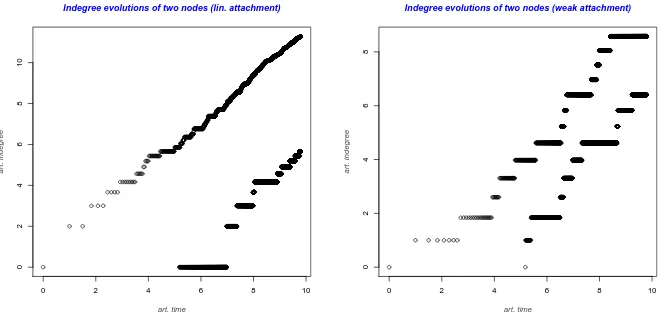
Figure 1: The degree evolution of a vertex in the artificial scaling: In the strong preference case, on the left, the distance of degrees is converging to a positive constant; in the weak preference case, on the right, fluctuations are bigger and, as time goes to infinity, the probability that the younger vertex has bigger degree converges to 1/2.
Proposition 1.12(Central limit theorem). In the case of weak preference, for all s∈T, Z[s,s+ϕκ∗t]−ϕ∗κt
p
κ : t ¾ 0
⇒(Wt:t ¾ 0),
in distribution on L[0,∞), where (Wt:t ¾ 0) is a standard Brownian motion and (ϕ∗t)t¾0 is the inverse of(ϕt)t¾0 given by
ϕt=
Z Φ−1(t)
0
1
f(u)2du.
We now briefly describe the background behind the findings above. In the artificial scaling, an in-degree evolution is the sum of a linear drift and a martingale, and the perturbations induced by the martingale are of lower order than the drift term. Essentially, we have two cases: Either the martingale converges almost surely, the strong preference regime, or the martingale diverges, the
weak preference regime. The crucial quantity which separates both regimes isP∞k=0f(k)−2with
con-vergence leading to strong preference. Its appearance can be explained as follows: The expected artificial time a vertex spends having natural indegree k is 1/f(k). Moreover, the quadratic vari-ation grows throughout that time approximately linearly with speed 1/f(k). Hence the quadratic variation of the martingale over the infinite time horizon behaves like the infinite sum above.
Investigations so far were centred aroundtypical vertices in the network. Large deviation princi-ples, as provided below, are the main tool to analyseexceptional vertices in the random network. Throughout we use the large-deviation terminology of Dembo and Zeitouni[1998]and, from this point on, the focus is on the weak preference case.
We set ¯f := f ◦Φ−1, and recall from Lemma A.1 in the appendix that we can represent ¯f as ¯
f(u) = uα/(1−α)¯ℓ(u) for u > 0, where ¯ℓ is a slowly varying function. This is the slowly varying function appearing in Theorem 1.8.
We denote byI[0,∞)the space of nondecreasing functionsx:[0,∞)→Rwithx(0) =0 endowed with the topology of uniform convergence on compact subintervals of[0,∞).
Theorem 1.13 (Large deviation principles). Under assumption (1), for every s ∈T, the family of functions
1
κZ[s,s+κt]:t ¾ 0
κ>0 satisfies large deviation principles on the spaceI[0,∞),
• with speed(κ1−1α¯ℓ(κ))and good rate function
J(x) =
(R∞ 0 x
α
1−α
t [1−˙xt+˙xtlog ˙xt]d t if x is absolutely continuous, ∞ otherwise.
• and with speed(κ)and good rate function
K(x) =
(
a f(0) if xt= (t−a)+for some a ¾ 0,
∞ otherwise.
Remark 1.14. The large deviation principle states, in particular, that the most likely deviation from the growth behaviour in the law of large numbers is having zero indegree for a long time and after that time typical behaviour kicking in. Indeed, it is elementary to see that a delay time ofaκhas a probability ofe−aκf(0)+o(κ), asκ↑ ∞.
More important for our purpose is a moderate deviation principle, which describes deviations on a finer scale. Similar as before, we denote byL(0,∞)the space of càdlàg functions x:(0,∞)→R
endowed with the topology of uniform convergence on compact subsets of(0,∞), and always use the conventionx0:=lim inft↓0xt.
Theorem 1.15 (Moderate deviation principle). Suppose(1) and that (aκ) is regularly varying, so
that the limit
c:=lim
κ↑∞aκκ 2α−1
1−α ¯ℓ(κ)∈[0,∞)
exists. Ifκ12−2−2αα¯ℓ(κ)−
1
2 ≪aκ≪κ,then, for any s∈T, the family of functions Z[s,s+κt]−κt
aκ :t ¾ 0
satisfies a large deviation principle onL(0,∞)with speed(a2κκ21α−−α1¯ℓ(κ))and good rate function
I(x) =
¨ 1 2
R∞
0 (˙xt)
2t1−ααd t−1
c f(0)x0 if x is absolutely continuous and x0 ¶ 0, ∞ otherwise,
where we use the convention1/0=∞.
Remark 1.16. If c = ∞ there is still a moderate deviation principle on the space of functions
x:(0,∞)→Rwith the topology of pointwise convergence. However, the rate functionI, which has the same form as above with 1/∞interpreted as zero, fails to be a good rate function.
Let us heuristically derive the moderate deviation principle from the large deviation principle. Let
(yt)t¾0denote an absolutely continuous path with y0 ¶ 0. We are interested in the probability that
PZ[s,s+κt]−κt
aκ ≈
yt=PZ[s,s+κt]
κ ≈t+
aκ
κ yt
.
Now note that x 7→1−x+xlogx attains its minimal value in one, and the corresponding second order differential is one. Consequently, using the large deviation principle together with Taylor’s formula we get
logP
Z[s,s+κt]−κt aκ ≈ yt
∼ −1
2κ
2α−1 1−α¯ℓ(κ)a2
κ
Z ∞
0
t1−αα˙y2
t d t−aκf(0)|y0|.
Here, the second term comes from the second large deviation principle. Ifcis zero, then the second term is of higher order and a path(yt)t¾0 has to start in 0 in order to have finite rate. Ifc∈(0,∞), then both terms are of the same order. In particular, there are paths with finite rate that do not start in zero. The casec=∞is excluded in the moderate deviation principle and it will not be considered in this article. As the heuristic computations indicate in that case the second term vanishes, which means that the starting value has no influence on the rate as long as it is negative. Hence, one can either prove an analogue of the second large deviation principle, or one can consider a scaling where the first term gives the main contribution and the starting value has no influence on the rate as long as it is negative. In the latter case one obtains a rate function, which is no longer good.
Remark 1.17. Under assumption (1) the central limit theorem of Proposition 1.12 can be stated as a complement to the moderate deviation principle: Foraκ∼κ
1−2α
2−2α¯ℓ(κ)−
1
2, we have Z[s,s+
κt]−κt
aκ :t ¾ 0
⇒q11−−2ααW
t11−−2αα:t ¾ 0
.
See Section 2.1 for details.
Proposition 1.18(Limit law for age and degree of the vertex of maximal degree). Suppose f satisfies assumption(1)and recall the definition of¯ℓfrom the paragraph preceding Theorem 1.13. Defining s∗t to be the index of the hub at time tone has, in probability,
s∗t ∼Z[s∗t,t]−t∼ 1
2 1−α
1−2α
t11−−2αα ¯
ℓ(t) =
1 2
1−α
1−2α
t
¯
f(t).
Moreover, in probability onL(0,∞),
lim
t→∞
Z[s∗
t,s∗t+tu]−tu
t11−−2αα¯ℓ(t)−1
:u ¾ 0
=
1−α
1−2α u
1−2α
1−α ∧1:u ¾ 0
.
The remainder of this paper is devoted to the proofs of the results of this and the preceding section. Rather than proving the results in the order in which they are stated, we proceed by the techniques used. Section 2 is devoted to martingale techniques, which in particular prove the law of large numbers, Proposition 1.10, and the central limit theorem, Proposition 1.12. We also prove absolute continuity of the law of the martingale limit which is crucial in the proof of Theorem 1.5. Section 3 is using Markov chain techniques and provides the proof of Theorem 1.1. In Section 4 we collect the large deviation techniques, proving Theorem 1.13 and Theorem 1.15. Section 5 combines the various techniques to prove our main result, Theorem 1.5, along with Proposition 1.18. An appendix collects the auxiliary statements from the theory of regular variation and some useful concentration inequalities.
2
Martingale techniques
In this section we show that in the artificial scaling, the indegree evolution of a vertex can be written as a martingale plus a linear drift term. As explained before, this martingale and its quadratic variation play a vital role in our understanding of the network.
2.1
Martingale convergence
Lemma 2.1. Fix s∈Tand represent Z[s,·]as
Z[s,t] =t−s+Mt.
Then(Mt)t∈T,t¾sis a martingale. Moreover, the martingale converges almost surely if and only if
Z ∞
0
1
f(u)2du<∞, (4) and otherwise it satisfies the following functional central limit theorem: Let
ϕt:=
Z Φ−1(t)
0
1
f(v)2 d v= Z t
0
1 ¯
and denote byϕ∗:[0,∞)→[0,∞)the inverse of(ϕt); then the martingales
converge in distribution to standard Brownian motion asκtends to infinity. In any case the processes
(1
Moreover, recalling the definition of the bracket〈M〉, e.g. from 12.12 in Williams[1991], we have
〈M〉t+∆t− 〈M〉t=
Observe that by Doob’sL2-inequality (see, e.g., 14.11 in Williams[1991]) and the uniform bound-edness of ¯f(·)−1 one has
whereC >0 is a constant only depending on f(0). Moreover, by Chebyshev’s inequality, one has
P
AsPak<∞, lettingitend to infinity, we conclude that almost surely
Note thatΦ:[0,∞)→[0,∞)is bijective and substituting(1−ǫ)κubyΦ(v)leads to
〈M〉t ¶ 1
1−ǫ
Z Φ−1((1−ǫ)(t−s))
0
1
f(v)2d v+η ¶
1 1−ǫ
Z Φ−1(t−s)
0
1
f(v)2d v+η.
Thus, condition (4) implies convergence of the martingale(Mt).
We now assume that(ϕt)t¾0 converges to infinity. Since ǫ >0 was arbitrary the above estimate implies that
lim sup
t→∞
〈M〉t
ϕt−s
¶ 1, almost surely.
To conclude the converse estimate note thatPt∈T(∆t)2<∞so that we get with (6) and (7) that
〈M〉t ¾
Z t−s
0
1
f(Φ−1((1+ǫ)u))du−η ¾
1 1+ǫ
Z Φ−1(t−s)
0
1
f(v)2d v−η,
for an appropriate finite random variableη. Therefore,
lim
t→∞
〈M〉t
ϕt−s
=1 almost surely. (8)
The jumps ofMκare uniformly bounded by a deterministic value that tends to zero asκtends to∞. By a functional central limit theorem for martingales (see, e.g., Theorem 3.11 in Jacod and Shiryaev [2003]), the central limit theorem follows once we establish that, for anyt ¾ 0,
lim
κ→∞〈M
κ
〉t=t in probability,
which is an immediate consequence of (8).
Proof of Remark 1.17. We suppose that f is regularly varying with indexα < 12. By the central limit theorem the processes
(Ytκ:t ¾ 0):=
Z[s,s+ϕ∗tϕ κ]−ϕ
∗
tϕκ p
ϕ(κ)
:t ¾ 0
forκ >0
converge in distribution to the Wiener process(Wt)asκtends to infinity. For eachκ >0 we consider the time change (τκt)t¾0 := (ϕκt/ϕκ). Using thatϕ is regularly varying with parameter 11−−2αα we
find uniform convergence on compacts:
(τκt)→(t11−−2αα) =:(τt) asκ→ ∞. Therefore,
Z[s,s+κt]−κt p
ϕ(κ)
:t ¾ 0= (Yτκκ
t :t ¾ 0)⇒(Wτt :t ¾ 0).
and, as shown in Lemma A.1,ϕκ∼ 11−−2αακ
1−2α
2.2
Absolute continuity of the law of
M
∞In the sequel, we consider the martingale(Mt)t¾s,t∈Tgiven by Z[s,t]−(t−s)for a fixeds∈Tin the case ofstrongpreference. We denote by M∞the limit of the martingale.
Proposition 2.2. If f is concave, then the distribution of M∞is absolutely continuous with respect to Lebesgue measure.
Proof. For ease of notation, we denoteYt=Z[s,t], for t∈T,t ¾ s. Moreover, we fixc>0 and let
At denote the event thatYu∈[u−c,u+c]for allu∈[s,t]∩T. Now observe that for two neighboursv−andvinS
P {Yt+∆t=v} ∩At
= (1−f¯(v) ∆t)P {Yt=v} ∩At+ ¯f(v−) ∆tP {Yt=v−} ∩At. (9) Again we use the notation ∆t = 1
Ψ−1(t). Moreover, we denote ∆f¯(v) = f¯(v)− f¯(v−). In the first
step of the proof we derive an upper bound for
h(t) =max
v∈S P {Yt =v} ∩At
fort ∈T,t ¾ s. With (9) we conclude that
P {Yt+∆t=v} ∩At
¶ (1−∆f¯(v) ∆t)h(t).
Forw ¾ 0 we denoteς(w) =maxS∩[0,w]. Due to the concavity of f, we get that
h(t+ ∆t) ¶ (1−∆¯f(ς(t+c+1)) ∆t)h(t). Consequently,
h(t) ¶ Y u∈[s,t)∩T
(1−∆f¯(ς(u+c+1)) ∆u)
and using that log(1+x) ¶ x we obtain
h(t) ¶ exp− X
u∈[s,t)∩T
∆f¯(ς(u+c+1)) ∆u
. (10)
We continue with estimating the sumΣin the latter exponential:
Σ = X
u∈[s,t)∩T
∆f¯(ς(u+c+1)) ∆u ¾
Z t
s
∆f¯(ς(u+c+1))du.
Next, we denote by flinthe continuous piecewise linear interpolation of f|N0. Analogously, we set
Φlin(v) =R0v flin1(u)du and ¯flin(v) = flin◦(Φlin)−1(v). Using again the concavity of f we conclude
that
Z t
s
∆f¯(ς(u+c+1))du ¾
Z t
s
(flin)′(Φ−1(u+c+1))du, and that
Hence,
Σ ¾
Z t
s
(flin)′(Φ−1(u+c+1))du ¾
Z t
s
(flin)′◦(Φlin)−1(u+c+1)du. For Lebesgue almost all arguments one has
(f¯lin)′= (flin◦(Φlin)−1)′= (flin)′◦(Φlin)−1·((Φlin)−1)′= (flin)′◦(Φlin)−1·flin◦(Φlin)−1
so that
(flin)′◦(Φlin)−1= (
¯
flin)′
¯
flin = (log ¯f lin)′.
Consequently,
Σ ¾ log ¯flin(t+c+1)−log ¯flin(s+c+1)
Using that flin ¾ f and(Φlin)−1 ¾ Φ−1we finally get that
Σ ¾ log ¯f(t+c+1)−logc∗,
wherec∗is a positive constant not depending on t. Plugging this estimate into (9) we get
h(t) ¶ c
∗
¯
f(t+c+1).
Fix now an intervalI⊂Rof finite length and note that
P {Mt∈I} ∩At
=P {Yt∈t−s+I} ∩At
¶ #[(t−s+I)∩S∩At]·h(t).
Now(t−s+I)∩S∩At is a subset of[t−c,t+c]and the minimal distance of two distinct elements
is bigger than ¯ 1
f(t+c). Therefore, #[(t−s+I)∩S∩At] ¶ |I|f¯(t+c) +1, and
P {Mt∈I} ∩At ¶ c∗|I|+ c
∗
¯
f(t+c).
Moreover, for any open and thus immediately also for any arbitrary intervalI one has
P {M∞∈I} ∩A∞ ¶ lim inf
t→∞ P {Mt∈I} ∩At
¶ c∗|I|,
where A∞ = Tt∈[s,∞)∩TAt. Consequently, the Borel measure µc on R given by µc(E) = E[1lA
∞1lE(M∞)], is absolutely continuous with respect to Lebesgue measure. The distribution µ
of M∞, i.e. µ(E) = E[1lE(M∞)], can be written as monotone limit of the absolutely continuous
measuresµc, asc↑ ∞, and it is therefore also absolutely continuous.
3
The empirical indegree distribution
In this section we prove Theorem 1.1. For k ∈ N∪ {0} and n ∈ N let µk(n) = E[Xk(n)] and µ(n) = (µk(n))k∈N∪{0}. We first prove part (a), i.e. that X(n) converges almost surely to µ, as n → ∞, in the total variation norm. To do this we associate the sequence (µ(n))n∈N to a time inhomogeneous Markov chain on N∪ {0}, which has µ as invariant measure. Then a coupling argument proves convergence ofµ(n)toµ, asn→ ∞. Finally, the almost sure convergence ofX(n)
is verified by a mass concentration argument based on the Chernoff inequality.
3.1
Proof of Theorem 1.1 (a)
Thus the linearity and the tower property of conditional expectation gives
µk(n+1) =µk(n) +
and conceivingµ(n)as a row vector we can rewrite the recursive equation as
µ(n+1) =µ(n)I+ 1 measure on the setN∪ {0}. Moreover, it is straightforward to verify that
f(0)µ0=1−µ0=
n+1Qto define an inhomogeneous Markov process. The entries
We denote for any admissible pairl,mby (Ynl,m)n¾m a Markov chain starting at time min state l
having transition kernels(P(n))n¾m. Due to the recursive equation we now have
µk(n) =P(Yn0,1=k).
Next, fixk∈N∪{0}, letm>karbitrary, and denote byνthe restriction ofµto the set{m,m+1, . . .}. Sinceµis invariant under eachP(n)we get
µk= (µP(m). . .P(n))k= mX−1
l=0
µlP(Ynl,m=k) + (νP
(m). . .P(n))
k.
Note that in the n-th step of the Markov chain, the probability to jump to state zero is 1
n+1 for all
original states in{1, . . . ,n−1}and bigger than n+11 for the original state 0. Thus one can couple the Markov chains(Ynl,m)and(Yn0,1)in such a way that
P(Ynl+,m1=Yn0,1+1=0|Ynl,m6=Yn0,1) = 1 n+1,
and that once the processes meet at one site they stay together. Then
P(Ynl,m=Yn0,1) ¾ 1−
n−1 Y
i=m
i
i+1−→1.
Thus(νP(m). . .P(n))k∈[0,µ([m,∞))]implies that
lim sup
n→∞
µk−P(Yn(0,1)=k) mX−1
l=0
µ∗l
¶ µ([m,∞)).
Asm→ ∞we thus get that
lim
n→∞µk(n) =µk.
In the next step we show that the sequence of the empirical indegree distributions(X(n))n∈N con-verges almost surely toµ. Note thatn Xk(n)is a sum ofnindependent Bernoulli random variables.
Thus Chernoff’s inequality (Chernoff[1981]) implies that for anyt>0
P Xk(n) ¶ E[Xk(n)]−t ¶ e−nt2/(2E[Xk(n)])=e−nt2/(2µk(n)).
Since
∞ X
n=1
e−nt2/(2µk(n))<∞,
the Borel-Cantelli lemma implies that almost surely lim infn→∞Xk(n) ¾ µk for allk∈N∪ {0}. If
A⊂N∪ {0}we thus have by Fatou’s lemma lim inf
n→∞
X
k∈A
Xk(n) ¾ X k∈A
lim inf
Noting thatµis a probability measure and passing to the complementary events, we also get
This establishes almost sure convergence of(X(n))toµin the total variation norm.
3.2
Proof of Theorem 1.1 (b)
We now show that the conditional law of the outdegree of a new node converges almost surely in the weak topology to a Poisson distribution. In the first step we will prove that, forη ∈(0, 1), and the affine linear attachment rule f(k) = ηk+1, one has almost sure convergence of Yn :=
Now note that due to Theorem 1.5 (which can be used here, as it will be proved independently of this section) there is a single node that has maximal indegree for all but finitely many times. Letm∗
denote the random node with this property. With Remark 1.11 we conclude that almost surely
logZ[m∗,n]∼lognη. (13)
Since for sufficiently largen
Yn=
Next, represent the incrementYn+1−Yn as
where ∆Mn+1 denotes a martingale difference. We shall denote by (Mn)n∈N the corresponding
martingale, that is Mn = Pnm=2∆Mm. Since 〈Y〉· is convergent, the martingale (Mn) converges almost surely. Next, we represent (14) in terms of ¯Yn = Yn− y as the following inhomogeneous
linear difference equation of first order:
One cannot split the sum into two sums since the individual sums are not summable. However, noticing that the individual term f(k)µkk≈ k2µk tends to 0, we can rearrange the summands to
obtain
〈µ, id〉= f(0)µ0+ ∞ X
k=1
f(k)µk=〈µ,f〉=η〈µ, id〉+1.
This implies that〈µ, id〉= y and that for anym∈N
〈X(n), 1l[m,∞)·id〉=〈X(n), id〉 − 〈X(n), 1l[0,m)·id〉 → 〈µ, 1l[m,∞)·id〉, almost surely.
Now, we switch to general attachment rules. We denote by f an arbitrary attachment rule that is dominated by an affine attachment rule fa. The corresponding degree evolutions will be denoted by(Z[m,n])and(Za[m,n]), respectively. Moreover, we denote byµandµathe limit distributions of the empirical indegree distributions. Since by assumption f ¶ fa, one can couple both degree evolutions such thatZ[m,n] ¶ Za[m,n]for alln ¾ m ¾ 0. Now
〈X(n),f〉 ¶ 〈X(n), 1l[0,m)·f〉+〈Xa(n), 1l[m,∞)·fa〉
so that almost surely
lim sup
n→∞ 〈
X(n),f〉 ¶ 〈µ, 1l[0,m)· f〉+〈µa, 1l[m,∞)·fa〉.
Sincemcan be chosen arbitrarily large we conclude that lim sup
n→∞ 〈X
(n),f〉 ¶ 〈µ,f〉.
The converse estimate is an immediate consequence of Fatou’s lemma. Hence,
lim
n→∞E
hXn
m=1
∆Z[m,n]
Fn
i
=〈µ,f〉.
Since, conditional onFn,Pnm=1∆Z[m,n]is a sum of independent Bernoulli variables with success probabilities tending uniformly to 0, we finally get thatL(Pnm=1∆Z[m,n]|Fn) converges in the weak topology to a Poisson distribution with parameter〈µ,f〉.
4
Large deviations
4.1
Exponentially good approximation
In order to analyze the large deviations of the processZ[s,·](orZ[m,·,]) we use an approximating process. We first do this on the level of occupation measures. Fors∈Tand 0 ¶ u<v we define
Ts[u,v) =sup{t′−t:Z[s,t] ¾ u,Z[s,t′]<v,t,t′∈T}
to be the time the processZ[s,·]spends in the interval[u,v). Similarly, we denote byTs[u]the time spent inu. Moreover, we denote by(T[u])u∈S a family of independent random variables with each entryT[u]beingExp(f(u))-distributed, and denote
T[u,v):= X w∈S
u¶w<v
T[w] for all 0 ¶ u ¶ v.
The following lemma shows thatT[u,v)is a good approximation to Ts[u,v)in many cases.
Lemma 4.1. Fixη1∈(0, 1), let s∈Tand denote byτthe entry time into u of the process Z[s,·]. One can couple(Ts[u])u∈S and(T[u])u∈S such that, almost surely,
1l{¯f(u)∆τ¶η1}|Ts[u]−T[u]| ¶ (1∨η2¯f(u))∆τ, whereη2 is a constant only depending onη1.
Proof. We fix t ∈ T with ¯f(u)∆t ¶ η1. Note that it suffices to find an appropriate coupling
conditional on the event{τ=t}. LetU be a uniform random variable and let F and ¯F denote the (conditional) distribution functions of T[u]and Ts[u], respectively. We couple T[u]andTs[u]by setting T[u] = F−1(U)and Ts[u] = F¯−1(U), where ¯F−1 denotes the right continuous inverse of ¯F.
The variablesT[u]andTs[u]satisfy the assertion of the lemma if and only if
F v−(1∨η2f¯(u))∆t
¶ F¯(v) ¶ F v+ (1∨η2f¯(u))∆t
for allv ¾ 0. (16) We compute
1−F¯(v) = Y t¶w,w+∆w¶t+v
w∈T
1−f¯(u)∆w=exp X
t¶w,w+∆w¶t+v u∈T
log 1−f¯(u)∆w
Next observe that, from a Taylor expansion, for a suitably large η2 > 0, we have −f¯(u)∆w−
η2 ¯f(u)2[∆w]2 ¶ log 1−f¯(u)∆w
¶ −f¯(u)∆w, so that
1−F¯(v) ¶ exp
−f¯(u) X t¶w,w+∆w¶t+v
w∈T
∆w
¶ exp −f¯(u)(v−∆t)=1−F(v−∆t).
This proves the left inequality in (16). It remains to prove the right inequality. Note that
1−F¯(v) ¾ exp− X
t¶w,w+∆w¶t+v w∈T
and
X
t¶w,w+∆w¶t+v w∈T
[∆w]2 ¶
∞ X
m=[∆t]−1
1
m2 ¶
1
[∆t]−1−1 ¶ ∆t.
Consequently, 1−F¯(v) ¾ exp{−f¯(u)(v+η2¯f(u)∆t)}=1−F(v+η2¯f(u)∆t).
As a direct consequence of this lemma we obtain an exponential approximation...
Lemma 4.2. Suppose that, for someη <1we have f(j) ¶ η(j+1)for all j∈N∪ {0}. If ∞
X
j=0 f(j)2
(j+1)2 <∞,
then for each s∈Tone can couple Tswith T such that, for allλ ¾ 0,
P sup
u∈S|
Ts[0,u)−T[0,u)| ¾ λ+p2K ¶ 4e−λ 2 2K,
where K>0is a finite constant only depending on f .
Proof. Fixs∈Tand denote byτu the first entry time of Z[s,·]into the stateu∈S. We couple the
random variablesT[u]andTs[u]as in the previous lemma and let, forv∈S,
Mv=X
u∈S
u<v
Ts[u]−T[u]=Ts[0,v)−T[0,v).
Then(Mv)v∈S is a martingale. Moreover, for each v = Φ(j)∈S one has τv ¾ Ψ(j+1) so that ∆τv ¶ 1/(j+1). Consequently, using the assumption of the lemma one gets that
∆τvf¯(v) ¶
1
j+1f(j) =:cv ¶ η <1.
Thus by Lemma 4.1 there exists a constant η′ <∞ depending only on f(0) andη such that the increments of the martingale(Mv)are bounded by
|Ts[v]−T[v]| ¶ η′cv.
By assumption we haveK:=Pv∈Sc2v <∞an we conclude with Lemma A.4 that forλ ¾ 0,
P sup
u∈S|
Ts[0,u)−T[0,u)| ¾ λ+p2K ¶ 4e−λ 2 2K.
We define(Zt)t¾0to be theS-valued process given by
Corollary 4.3. In distribution on the Skorokhod space, we have
lim
s↑∞(Z[s,s+t])t¾0= (Zt)t¾0.
Proof. Recall that Lemma 4.1 provides a coupling between(Ts[u])u∈S and(T[u])u∈S for any fixed
s ∈T. We may assume that the coupled random variables (T¯s[u])u∈S and (T¯[u])u∈S are defined
on the same probability space for alls∈T(though this does not respect the joint distributions of
(Ts[u])u∈Sfor different values ofs∈T). Denote by(Z¯[s,·])s∈Tand(Z¯t)the corresponding processes such that ¯Ts[0,u) +s=s+Pv<uT¯s[v]and ¯T[0,u) =Pv<uT¯[v]are the entry times of(Z¯[s,s+t])
and(Z¯t)into the stateu∈S. By Lemma 4.1 one has that, almost surely, lims↑∞T¯s[0,u) = T¯[0,u)
and therefore one obtains almost sure convergence of(Z¯[s,s+t])t¾0 to(Z¯t)t¾0 in the Skorokhod
topology, which implies the stated convergence in distribution.
Proposition 4.4. Uniformly in s, the processes
• (1κZκt:t ¾ 0)κ>0and(κ1Z[s,s+κt]:t ¾ 0)κ>0;
• (1
aκ(Zκt−κt):t ¾ 0)κ>0 and( 1
aκ(Z[s,s+κt]−κt):t ¾ 0)κ>0,
are exponentially equivalent on the scale of the large, respectively, moderate deviation principles.
Proof. We only present the proof for the first large deviation principle of Theorem 1.13 since all other statements can be inferred analogously.
We let Uδ(x) denote the open ball around x ∈ I[0,∞) with radius δ >0 in an arbitrarily fixed
metric d generating the topology of uniform convergence on compacts, and, for fixed η > 0, we cover the compact set K ={x ∈ I[0,∞):I(x) ¶ η} with finitely many balls(Uδ(x))x∈I, where
I⊂K. Since every x ∈Iis continuous, we can findǫ >0 such that for every x ∈Iand increasing and right continuousτ:[0,∞)→[0,∞)with|τ(t)−t| ¶ ǫ,
y∈Uδ(x) ⇒ yτ(·)∈U2δ(x).
For fixed s ∈ T we couple the occupation times (Ts[0,u))u∈S and (T[0,u))u∈S as in Lemma 4.2, and hence implicitly the evolutions (Z[s,t])t¾s and (Zt)t¾0... Next, note that Z[s,s+ ·] can be
transformed into Z· by applying a time change τ with |τ(t)− t| ¶ supu∈S|Ts[0,u)−T[0,u)|. Consequently,
P d 1κZ[s,s+κ·],1κZκ·
¾ 3δ ¶ P1
κZκ·6∈
[
x∈I Uδ(x)
+Psup
u∈S|
¯
Ts[0,u)−T¯[0,u)| ¾ κǫ
,
and an application of Lemma 4.2 gives a uniform upper bound ins, namely
lim sup
κ→∞
sup
s∈S
1
κ1−1α¯ℓ(κ)
logP d κ1Z[s,s+κ·],1κZκ·
¾ 3δ ¶ −η.
4.2
The large deviation principles
By the exponential equivalence, Proposition 4.4, and by [Dembo and Zeitouni, 1998, Theorem 4.2.13] it suffices to prove the large and moderate deviation principles in the framework of the exponentially equivalent processes (17) constructed in the previous section.
The first step in the proof of the first part of Theorem 1.13, is to show a large deviation principle for the occupation times of the underlying process. Throughout this section we denote
aκ:=κ1/(1−α)¯ℓ(κ).
We define the functionξ:R→(−∞,∞]by
ξ(u) =
(
log11
−u ifu<1,
∞ otherwise.
Its Legendre-Fenchel transform is easily seen to be
ξ∗(t) =
(
t−1−logt if t>0,
∞ otherwise.
Lemma 4.5. For fixed0 ¶ u<v the family(1
κT[κu,κv))κ>0satisfies a large deviation principle with
speed(aκ)and rate functionΛ∗u,v(t) =supζ∈R[tζ−Λu,v(ζ)], where
Λu,v(ζ) =
Z v
u
s1−ααξ(ζs−α/(1−α))ds.
Proof. For fixedu<v denote byIκ=Iκ[u,v)={j∈N∪ {0}:Φ(j)∈[κu,κv)}. We get, using(Sj)for
the underlying sequence ofExp(f(j))-distributed independent random variables,
Λκ(θ):= logEeθT[κu,κv)/κ
= X
j∈Iκ
logEeθκSj=X j∈Iκ
log 1
1−κfθ(j) =
X
t∈Φ(Iκ)
ξ θ
κf(Φ−1(t))
=
Z
¯ Iκ
f(Φ−1(t))ξ θ
κf(Φ−1(t))
d t,
where ¯Iκ=¯Iκ[u,v)=Sj∈I
κ[Φ(j),Φ(j+1)). Now chooseθ in dependence onκasθκ=ζκ
1/(1−α)¯ℓ(κ)
withζ <uα/(1−α). Then
Z
¯Iκ
¯
f(t)ξ θκ κf¯(t)
d t=κ
Z
¯Iκ/κ
¯
f(κs)ξ θκ κf¯(κs)
ds
=κ1/(1−α)
Z
¯Iκ/κ
s1−αα¯ℓ(κs)ξ
ζ¯ℓ(κ)
s1−αα¯ℓ(κs)
Note that inf¯Iκ/κand sup¯Iκ/κapproach the valuesuandv, respectively. Hence, we conclude with the dominated convergence theorem that one has
Λκ(θκ)∼κ1/(1−α)¯ℓ(κ)
Z v
u
s1−ααξ( ζ
s1−αα)ds
| {z }
=Λu,v(ζ)
as κtends to infinity. Now the Gärtner-Ellis theorem implies the large deviation principle for the family(T[κu,κv))κ>0 for 0< u< v. It remains to prove the large deviation principle foru= 0. Note that
ET[0,κv) =EX
j∈Iκ Sj=
Z
¯ Iκ
f(Φ−1(t)) 1
f(Φ−1(t))d t∼κv
and
var(T[0,κv)) =X j∈Iκ
var(Sj) =
Z
¯Iκ
f(Φ−1(t)) 1
f(Φ−1(t))2d t®
1
f(0)κv.
Consequently, T[0,κκǫ) converges in probability toǫ. Thus for t<v
Pκ1T[0,κv) ¶ t
¾ Pκ1T[0,κǫ) ¶ (1+ǫ)ǫ
| {z }
→1
P1κT[κǫ,κv) ¶ t−(1+ǫ)ǫ
and for sufficiently smallǫ >0
lim inf
κ→∞
1
aκ
logPκ1T[0,κv) ¶ t ¾ −Λ∗ǫ,v(t−(1+ǫ)ǫ),
while the upper bound is obvious.
The next lemma is necessary for the analysis of the rate function in Lemma 4.5. It involves the functionψdefined asψ(t) =1−t+tlogt fort ¾ 0.
Lemma 4.6. For fixed0<x0<x1there exists an increasing functionη:R+→R+withlimδ↓0ηδ=0
such that for any u,v∈[x0,x1]withδ:=v−u>0and all w∈[u,v],t>0one has
Λ∗u,v(t)−w
α
1−αtψ δ
t
¶ ηδ
δ+tψ δt
.
We now extend the definition ofΛ∗continuously by setting, for anyu ¾ 0 and t ¾ 0,
Λ∗u,u(t) =u1−ααt.
For the proof of Lemma 4.6 we use the following fact, which can be verified easily.
Lemma 4.7. For anyζ >0and t>0, we have|ξ∗(ζt)−ξ∗(t)| ¶ 2|ζ−1|+|logζ|+2|ζ−1|ξ∗(t). Proof of Lemma 4.6. First observe that
γδ:= sup
x0<u<v<x1
v−u¶δ
tends to 1 asδtends to zero. By Lemma 4.7, there exists a function(η¯δ)δ>0with limδ↓0η¯δ=0 such
that for allζ∈[1/γδ,γδ]andt>0
|ξ∗(ζt)−ξ∗(t)| ¶ η¯δ(1+ξ∗(t)).
Consequently, one has for anyδ >0, x0<w, ¯w<x1 with|w−w¯| ¶ δandζ∈[1/γδ,γδ]that
|w¯1−ααξ∗(ζt)−w α
1−αξ∗(t)| ¶ w¯ α
1−α|ξ∗(ζt)−ξ∗(t)|+ξ∗(t)|w¯ α
1−α −w α
1−α|
¶ cη¯δ(1+ξ∗(t)) +cδξ∗(t),
wherec<∞is a constant only depending onx0,x1andα. Thus for an appropriate function(ηδ)δ>0
with limδ↓0ηδ=0 one gets
|w¯1−ααξ∗(ζt)−w α
1−αξ∗(t)| ¶ ηδ(1+ξ∗(t)). (18) Fixx0<u<v<x1 and setδ:=v−u. We estimate, forθ ¾ 0,
δu1−ααξ(θv−α/(1−α)) ¶ Λu,v(θ) ¶ δv
α
1−αξ(θu−α/(1−α)), and the reversed inequalities forθ ¶ 0. Consequently,
Λ∗u,v(δt) =sup
θ
[θt−Λu,v(θ)]
¶ δsup
θ
[θt−u1−ααξ(θv−α/(1−α))]∨δsup
θ
[θt−v1−ααξ(θu−α/(1−α))]
=δu1−ααξ∗((v/u) α
1−αt)∨δv α
1−αξ∗((u/v) α
1−αt).
Since(v/u)α/(1−α)and(u/v)α/(1−α)lie in[1/γδ,γδ]we conclude with (18) that forw∈[u,v)
Λ∗u,v(δt) ¶ w1−ααξ∗(t)δ+ηδ(1+ξ∗(t))δ. To prove the converse inequality, observe
Λ∗u,v(t) ¾
δsup
θ¶0
[θt−u1−ααξ(θv−α/(1−α))]
∨
δsup
θ¾0
[θt−v1−ααξ(θu−α/(1−α))]
.
Now note that the first partial Legendre transform can be replaced by the full Legendre transform if t ¶ (u/v)α(1−α). Analogously, the second partial Legendre transform can be replaced if t ¾ (v/u)α(1−α). Thus we can proceed as above ift6∈(1/γδ,γδ)and conclude that
Λ∗u,v(t) ¾ w1−ααξ∗(t)δ−ηδ(1+ξ∗(t))δ.
The latter estimate remains valid on(1/γδ,γδ)if x α/(1−α)
1 (ξ∗(1/γδ)∨ξ∗(γδ)) ¶ ηδ. Sinceγδtends
to 1 and ξ∗(1) = 0 one can make ηδ a bit larger to ensure that the latter estimate is valid and
limδ↓0ηδ=0. This establishes the statement.