DIAGRAME FOR A SOFTWARE PID
by
Valentin Casavela
Abstract.The software PID, shown below, is designated for to command an inverter, inverter used to vary the speed of an induction motor. The C++ program was descriebed in [3] and outs a byte on the parallel interface, that is the output data register. From this byte, six bits are used to command an interface, built in six channels, every channel commanding the gate of one of six IGBT-s. Every phase of the inverter needs two IGBT-s. The speed of the motor is read on the status register, of the same parallel interface.To enhance the performance, an algorithm with superior performance is adapted from the direct software Pulse Width Modulation (PWM) approach
Keywords.Pulse Width Modulation.Isolate Bipolar Transistors. Parallel interface.
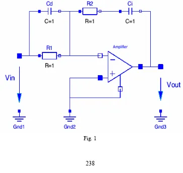
[image:1.595.126.489.314.657.2]Model for Software PID. The implementation of software PID control was performed in our laboratory. The beginning is the hardware PID, which scheme is designed in figure 1.
Generally, the PID control has a potential ability to control the output of a process variable. If the control constants are chosen correctly, the variable approaches and maintains a desired value, its set point. This variable could be a temperature, a reactor conversion, the effluent conversion in a separation, etc. Our case is the speed of an induction motor.
These controllers can be implemented mechanically, by hard-wired electronics or within the software of a computer. Labview program may be used to accomplish control too. The purpose of this article is to show the general diagram, which may be implemented in Labview or in C++ software program. PID control starts by measuring the variable that is to be controlled. This is accomplished by an A to D (Analog to Digital) converter. This measures a voltage or current and outputs a numerical value to the computer, corresponding to this measurement. These measurements are typically 8,12 to 16 bits and are measured many times per second.
Based in the control operation, a voltage is set by the use of a D to A (Digital to Analog) converter. This sets the voltage or current to an electronic component, based on a variable chosen in software inside the computer program. The basic equation which reflects PID control uses the difference between a measured voltage, VD, and the setpoint , SP, to set a desired voltage, Vout. See fig1.
p D
in V S
V = −
First, on calculate impedance:
( )
( )
( )
( )
( )
( )
( )
( )
( )
1 1( )
;...(1) ;... ;.. ;... : ,.... 1 1 , ;... ;... 1 ;... 1 1 * 2 2 1 1 2 1 2 1 2 2 1 1 2 1 2 2 1 1 1 2 2 2 1 1 1 s V s T s T K s V C R C R C C R R T C R C R T C R C R C R K where s T s T K s H Finally s Z s Z s V s V s H s C R s Z s C R s C R s Z IN D I R out D I R D I R IN out I d d + + = + = + = + − = + + = − = = + = + =pole, near the zero, created by derivation time Td. So, the excessive growing and noise, due the derivation, will be attenuated.
For our next proposes, it doesn’t matter, the corresponding physical modification into figure 1. Expression 1 becomes:
( )
( )
;...(2) 11
1 V s
s T s T s T K s
V D IN
I R out + + + = ε
The next step is passing to the digital form, using the sample theorem and Z transformation. For that, there are two possibilities: 1) rectangles method and 2) trapezium method.
1) For that,
) 3 ....( ... ... ... ... ... ... * 1 .... ;. 1 .. ),.. 1 ( 1 ) )( ( ) ( ,.. ;... ln } ( .. ;.. 0 0 0 ' Z T Z s finally e Z for Z Z Z Z z f Z f so Z Z f note Z esT − = = = − = − = = =
It will replace "s", witch multiplies
T
D..
and
..
T
ε in (2), and2) Likewise, in trapezium method,
1
1
*
2
+
−
=
Z
Z
T
s
. It will replace"s", witch multipliesI
T in (2).
T is sample time and is infinitesimal short. Trapezium method is used for slow variations, like integration (TI ), but rectangles method is used for speed variation, like derivation (TD ).
Now, the digital transfer function may be obtain:
)
4
..(
]...
)
1
(
1
*
1
1
*
2
1
[
T
T
T
T
Z
Z
T
T
Z
Z
T
T
K
D
D I R PID ε ε−
+
−
+
−
+
+
=
After some processing,
Our software PID regulator has input as error e(k)=ΩP- Ωm, where ΩP is imposed angular velocity and Ωm is measured angular velocity, for an induction motor.
The measurement for Ωm is made with a transducer, a disk fixed on the motor ax, which disk has “n” halls and “n” full. Passing from a hall to a full determines a pulse, read by the system in a preset time. So Ωm is measured.
ΩP is the imposed angular velocity, by user program. To the inverter and, finally, to the motor comes, as a command, the calculated angular velocity: ΩC, given by formula:
) 6 );...( 2 ( )
1 ( ) 1 ( ) 2 ( ) 1 ( ) ( )
( = + 1 − + 2 − + − 1 Ω − + 1Ω − ΩC K dOe K de K d e k c C K c c K
dI and cI are given by (5) and e(k-i), Ω(K-i) are given by multiplying with z-I
ΩC is, in fact, Vout and “e” is Vin, in expression (2), but at discreet times.
ΩC=2π*fC, where fC is the resulting frequency for the stator rotating magnetic field. The real (and measured velocity) is Ωm, related Ωc by expression:
Ωm=(1-s) ΩC
“s” is the slide for the induction motor. For according the software PID [2], with the system, formed by inverter-motor, the transfer functions of the last:
Ks= Ωm/ ΩC=1-s,
must be equal with that given by (2) expression: Vout/Vin .
For the same purpose, the according, in (1) and (2) expressions, we must impose [2]:
)
7
...(
;...
2
;...
)
2
(
2
;...
*
2
.
1
2
T
T
T
T
T
T
T
T
T
T
T
K
K
uD U
u I
u a
S R
+
=
+
+
=
+
=
Diagram for Software PID Implementation
The diagram is shown below.
2
regulator()
Ti
←
2*(Tu+T/2)/(Tu+T)
Td
←
(Tu+T)/2
Tp
←
Per/10000
fp
←
1/Tp
nmas
Å
0, measured turation ; ek
Å
0, error
Perp(imposed period) = = Per
i < = sample
i=0
N
Y
3
return
6
Ks
←
1-s
Kr
←
(1.2/Ks)*(Ta/(Tu+T))
omegap
←
2*pi*fp/p
nmas
←
0
tradperiod>0
Y
N
nmas
←
10 000/(2*n*tradperiod), rot/s
omegam
←
2 pi*nmas
ek
←
omegap-omegam
d0
←
(Kr/(1+Tniu/T))*(1+(T+Tniu)/(2*T)+(Td+Tniu)/T)
d1
←
(Kr/(1+Tniu/T))*(1+T/(2*T)-2*(Td+Tniu)/T)
d2
←
(Kr/(1+Tniu/T))*((T+Tniu)/T-Tniu/(2*T))
c1
←
–Tniu/(T+Tniu)
omegack=d0*ek+d1*ek1+d2*ek2+(1-c1)*omegack1+c1*omegack2
3
REFERENCES:
1)Teodor Pana: “Controlul sistemelor de actionare vectoriala cu motoare de inductie—Editura Mediamira, cluj-napoca, 2001
2) I. Cioc,C. Nica: “Proiectarea masinilor electrice”-Editura Pedagogica,1994
3) Valentin Casavela: P.W.M., Software P.I.D. and Command Transmission, Implemented in C++,for Induction Machine, International Conference of Automation, Quality and Tasting, Robotics, May 23-25, 2002, University of Girona.
Author:
Valentin Casavela, University of Petrosani, e-mai [email protected], [email protected]
Per
←
10000/fc
Amp
←
10000/Per
ek2
←
ek1
ek1
←
ek
omegack2
←
omegack1
omegack1
←
omegack
s
←
(omegac-omegam)/omegac
ek*ek>epsilon
Y
N
i++
Per
Å
Perp