www.elsevier.nlrlocatereconbase
‘Competition’ among employers offering health
insurance
David Dranove
a,), Kathryn E. Spier
a, Laurence Baker
b,ca
Northwestern UniÕersity, EÕanston, IL, USA b
Stanford UniÕersity, Stanford, CA, USA
c ( )
National Bureau of Economic Research NBER , USA
Accepted 15 March 1999
Abstract
Most employees contribute towards the cost of employer-sponsored insurance, despite tax laws that favor zero contributions. Contribution levels vary markedly across firms, and
Ž .
the average contribution as a percentage of the premium has increased over time. We offer a novel explanation for these facts: employers raise contribution levels to encourage their employees to obtain coverage from their spouses’ employer. We develop a model to show how the employee contribution required by a given firm depends on characteristics of the firm and its work force, and find empirical support for many of the model’s predictions. q2000 Elsevier Science B.V. All rights reserved.
JEL classification: I11; J33
Keywords: Health insurance; Employer; Employee
1. Introduction
Since the 1950s, most Americans under 65 have obtained health insurance
Ž .
through their employers Employee Benefit Retirement Institute, 1995 . While it is commonplace today for workers and employers to contribute jointly towards the
)Corresponding author. Kellogg Graduate School of Management, 2001 Sheridan Road, Evanston, IL 60208. Tel.:q1-847-491-8682; Fax:q1-847-467-1777; E-mail: [email protected]
0167-6296r00r$ - see front matterq2000 Elsevier Science B.V. All rights reserved.
Ž .
cost of these plans, there is tremendous variation in these contributions across firms.1 While some firms continue to pay the entire cost of insurance, others require contributions towards individual coverage of US$500 or more, and contri-butions towards family coverage of US$2500 or more. There has also been an increase in employee contributions over time. As recently as 1980, the majority of
Ž
employers bore the entire cost of health insurance Employee Benefit Retirement
.
Institute, 1995 .
We argue that these patterns of health insurance contributions may be driven, at least in part, by the presence of two-career couples and employer competition to be the ‘employer not chosen’ for insurance. We present a model in which competitive forces lead employers to raise contributions to encourage their work-ers to switch plans and obtain insurance from their spouses’ employwork-ers instead.2 We show that the equilibrium employee contribution is sensitive to several critical factors, including the cost of insurance, the percentage of two-career couples, the income tax rate, and the heterogeneity of plans and employee preferences. Using data from the Robert Wood Johnson Foundation Employer Health Insurance Survey, we find empirical support for several key predictions of our model.
Our analysis is motivated by a fundamental difference that exists between health insurance and other employee benefits. Namely, family health insurance benefits obtained by different members of a household generally substitute for one another, whereas pensions, life insurance, and other benefits obtained by different members of a household generally augment one another. The implication is that firms can reduce their health insurance costs without necessarily reducing the well-being of their employees by encouraging them to obtain coverage from their spouses’ employers.
Although we have heard numerous anecdotes supporting our explanation for why employers require employees to make contributions towards health insurance,
Ž .
we have seen no discussion of it in the literature. Morrisey et al. 1994 note that small employers require larger contributions than do large employers but offer no explanation for either the imposition of contributions or the differential. They also report that insurance offered by small employers is less generous on other dimensions besides contribution levels. While our model focuses on contributions, the intuitions that we draw should apply to these other dimensions as well. That is, firms may reduce the generosity of insurance so as to encourage their employees to select their spouse’s plans. The savings would offset the foregone tax benefits of providing more generous insurance to those workers who do not switch plans.
1
Using data from the Robert Wood Johnson Foundation Employer Health Insurance Survey, we find that the coefficient of variation of contributions towards family plans is approximately 0.75.
2
In the theoretical part of our paper, some employees have low demand for insurance from their own employer because they have the option of obtaining insurance through their spouse’s employer. Firms select contribution levels to trade off the tax advantages of employer contributions and the savings from shifting coverage onto other employers. As in the classic economic model of how tax considerations distort individuals’ decisions to purchase health insurance, employers may increase contributions to discourage insurance purchases by em-ployees with low demand for insurance.3 Our model differs from this standard model, however, because employer-specific demand is endogenous and depends on the contracts offered in equilibrium. Several important results are obtained. First, employee contributions are lower when fewer employees have working spouses. Second, we show that firms with low insurance premia require dispropor-tionately lower contributions in equilibrium and identify a potential source of welfare loss associated with this divergence in insurance offerings.
We are able to test some of the predictions of our theoretical model with data drawn from the Robert Wood Johnson Foundation Employer Health Insurance Survey, conducted by Rand and Westat in late 1993 and early 1994. First, we find that larger firms generally require smaller contributions, especially when measured in percentage terms. This is consistent with our theoretical result that firms that have higher costs of insurance tend to have disproportionately higher tions. Second, we find that firms with more female workers have higher contribu-tions, firms with more male workers over age 55 have lower contribucontribu-tions, and firms with more covered part time workers have higher contributions. These findings are consistent with our prediction that contributions should be higher in firms with a higher the percentage of working spouses.
Simulations of our model show that even small increases in the percentage of dual-worker households can help to account for the rapid increase in contributions that have occurred over the past few decades. There are other factors that have contributed to the growth of employee contributions over time, however, and we do not pretend that our explanation is the main one. One factor is the growth of benefit plans that enable employees to contribute towards premia with before-tax dollars. Between 1988 and 1993, the percentage of medium to large employers offering flexible spending accounts that might enable employees to make contribu-tions with before-tax dollars increased from 13% to 53%. Another explanation may be that as employers offer more insurance options to their employees, they are requiring contributions towards more expensive plans to try to shift employees into the less expensive ones. Although this explanation is consistent with the rise in contributions to individual plans, it does not explain why an increasing
3 Ž . Ž .
percentage of firms require their employees to make non-trivial contributions to even their least expensive plans.
Ž .
Levy 1998 examines the same question. She hypotheses that firms use employee contributions to distinguish between workers with different demands for health insurance, in order to provide optimal compensation when workers are mobile and recruiting workers is costly. Like us, she argues that firms will increase contribution levels so as to discourage workers with low demand for health insurance from purchasing it. In her model, the firm then rewards workers with higher wages so as to discourage them from changing jobs. In our model, firms offer symmetrical wagerbenefit packages so that workers are indifferent between jobs. Levy finds some empirical support for her hypothesis, but it does not appear to fully explain variation in contributions in the cross-section or over time.
Section 2 introduces the basic model of firms with identical insurance costs and derives the basic results. Section 3 extends this model to consider heterogeneous firms with different costs of insurance. Section 4 provides some empirical support for the model. Section 5 offers concluding remarks.
2. The symmetric model
In our model, firms compete for workers in a perfectly competitive labor market. For simplicity, we assume all workers are married, and that all insurance policies are for ‘family coverage’ where both husband and wife are covered by the policy. In order to focus on competition between employers, we assume that all employees have sufficiently high demand for insurance that they will purchase insurance through either their own employer or their spouse’s employer regardless of contribution levels.4 Labor contracts specify both a wage, W, and the worker’s contribution for family health coverage, C. In other words, the worker pays C if he decides to purchase his family’s insurance through his employer. The cost of
Ž .
insurance to the firm is P the ‘premium’ for each family covered. Each
4
employer offers identical employment contracts, W, C , to all their employees. In
U U
4
this section we construct a symmetric equilibrium, W , C , in which all firms offer the same wage and benefits packages. Not only is the symmetric model analytically tractable and generates clear predictions, it also provides the analytic framework for the richer asymmetric framework that follows. The drawback is that
4
it does not allow for otherwise identical firms to sort themselves by insurance offerings.5
To generate a symmetric equilibrium we assume that at the time they select their employer, workers do not know whether their spouses will work. Specifi-cally, with probability a, a worker will have a working spouse, and with probability 1ya the spouse will not be working.6 This implies that when they select employers, the workers do not know the nature of the insurance package
Ž .
that their spouses may receive and therefore do not know their own long-run preferences for insurance. This not only permits a symmetric equilibrium, but is also realistic for many workers.7Some workers choose job market strategies early in their careers before many other aspects of their lives have been resolved—par-ticularly marriage, whether their spouse will be in the labor market, and what kind of job their spouse will ultimately settle into. Other workers in stable job situations have spouses who may move in and out of the labor market over time. Again, this generates uncertainty about the value of benefits.
Formally, the utility that a person gets from consuming a health care plan is stochastic.8 First imagine that two agents, 1 and 2, are married and both are employed. If they opt for agent 1’s health care plan, agent 1 receives a payoff of
´11
and agent 2 receives a payoff of ´21
. More generally, if agent i is covered by agent j’s plan, his payoff is ´i j
. The payoff ´i j
is measured in dollars. We assume that these payoffs are i.i.d. with sufficiently large mean that essentially all individuals purchase insurance at prevailing prices.9 So if agents 1 and 2 are married with respective contributions of C1 and C2, they will accept agent 1’s policy instead of agent 2’s if and only if ´11q´21yC1G´12q´22yC2, or
´11
q´21
y´12
y´22
GC1yC2.
Ž .
1Let zs´11q´21y´12y´22. This random variable represents the dollar value of a married couple’s preference for agent 1’s health plan over agent 2’s. Given our assumption that each ´i j is i.i.d., we know that z is symmetric with a zero
5 Ž .
Scott et al. 1989 show that workers with heterogeneous demands for benefits may sort
Ž .
themselves across firms or across job types within firms to obtain their most preferred wagerbenefit package.
6
This framework could be easily adapted to consider the case where the worker does not know
Ž
whether he will be working in the future so the worker and the spouse would be symmetric in this
.
regard .
7 Ž .
Lazear 1995 provides evidence that suggests that workers may be unlikely to change jobs upon discovering the particulars of their spouse’s benefits package. He reports that while 20% of new hires change employers within a year, only 2% of workers who have been with a firm five or more years will change jobs during the year. Lazear suggests that this search is based on a matching of worker skills to employer needs. By inference, job switching is not a response to spousal benefit opportunities.
8
This assumption is necessary to derive an equilibrium in which wages and contributions are continuous functions of the parameters of the model.
9
Ž . Ž .
mean. Let h z denote the probability density function, and H z represent the
Ž .
cumulative distribution function, of the left-hand side of inequality 1 .
4
At the time when a worker is considering a job with a contract W,C , he has
U U4 10 the option of accepting another job with equilibrium characteristics W ,C .
4 Ž
Suppose that a firm offers this worker an alternative contract, W,C , where for
. U U
example W)W and C-C , so that the firm offers a lower contribution level but a higher base wage than the market standard. The worker would be willing to accept this new contract if the following condition is satisfied:
w
Ux
w
Ux
11 21 121yt WyW y 1ya CyC qa E ´ q´ yC,´
Ž
.
Ž
.
ma xŽ
q´22
yCU yE ´11
q´21
yCU,´12
q´22
yCU G0. 2
.
maxŽ
.
4
Ž .
Ž . Ž 11 21 12 22 . Ž U U.
Let G a, b denote Emax ´ q´ ya, ´ q´ yb . Then G C ,C
de-notes the expected benefit of insurance to an individual who has two insurance
U Ž U.
options each with contribution level C . SimilarlyG C,C denotes the expected benefit of insurance to an individual with two insurance options, one of which requires contribution level C and the other of which requires CU. We can rewrite
Ž .
Eq. 2 as
w
Ux
w
Ux
1yt WyW y 1ya CyC
Ž
.
Ž
.
qa G
Ž
C,CU.
yGŽ
CU,CU.
4
G0.Ž .
3 The expression is interpreted as follows. The first term represents the difference in the worker’s after tax income, which the worker enjoys whether or not his spouse works. The second term represents the offsetting change in the insurance contribution in the case where his spouse does not work in the future. The final term represents the offsetting change in the contribution in the event that the spouse does work in the future. This captures the fact that the worker and his spouse may prefer to purchase the insurance with the higher contribution level due to their idiosyncratic evaluations.Solving for W as a function of C, we have:
U U
WGW q 1r
Ž
1yt. Ž
1ya. Ž
CyC.
U U U
ya G
Ž
Ž
C,C.
yGŽ
C ,C.
.
.Ž .
4In other words, for any contribution, C, this expression tells us that the corre-sponding base wage must be at least this large. If the base wage fell short of this level, then the worker would not be willing to accept the position.
10 U U4
We will take W ,C as given for now, and then solve for a symmetric equilibrium in which
4 U U4
U U
4
If the other firms in the economy are offering standard packages of W ,C , the best package that a firm could offer solves the following program:
U
Min Wq
Ž
PyC. Ž
1ya.
qa 1yH CŽ
yC.
4
,W ,C4
s.t. Eq. 4 and C
Ž .
G0.The firm wants to minimize the total cost of employing a worker, subject to the
Ž
constraints that the worker be willing to accept the job this individual rationality
Ž ..
constraint is given by Eq. 4 and that the contribution level is non-negative.
ŽNegative contributions would simply be transfers from the employer to the
.
employee and would be legally taxable. The costs include the base wage, W, plus
Ž .
the employer’s contribution to the health insurance premium, PyC . This is borne by the employer in two situations: if the agent’s spouse is non-working,
Ž .
which occurs with probability 1ya , and in the situation where the spouse is working but opts for the employer’s plan. This latter case occurs with probability
w Ž U.
x
a 1yH CyC .
By raising its contribution level sufficiently so as to encourage its employees to choose their spouses’ insurance, an employer avoids the cost of insurance. Employees with working spouses may benefit from the higher contributions when the corresponding higher wages more than offset the potential tax benefit. But it harms employees with stay-at-home spouses who no longer enjoy the tax benefit of generous insurance. The ‘right’ contribution level balances the preferences of employees with working spouses and employees with stay-at-home spouses.
U U4
Lemma: If workers have an outside option of receiving contract W ,C , the
Ž U.
best employment contract a firm can offer has a contribution Csw a,t,C
Ž . Ž . w Ž .xŽ Ž U.. Ž
implicitly defined by 1ya r1yt y ar1yt 1yH CyC y 1y
Ž U.. Ž . Ž U.
aH CyC y PyC ah CyC s0 if CG0, and Cs0 otherwise.
Proof: See Appendix A.
By first considering the case where nobody has a working spouse we can understand the tradeoffs facing the firm. If as0, then the first order condition
Ž .
reduces to 1r1yt y1 which is positive for all positive t. Thus, the firm would like to decrease the contribution as much as possible. This reflects the familiar result that when benefits are tax exempt, the firm gives benefits instead of wages. Now suppose that some spouses are employed, so a)0, and that the solution
Ž U.
has Csw a,t,C )0. If the firm raises the contribution level, there are two
Ž . Ž . w Ž .xŽ
main effects. The first effect, given by the terms 1ya r1yt y ar1yt 1
Ž U..
yH CyC is the increase in wages necessary to offset the decrease in utility to those individuals with and without working spouses respectively. The benefit to
Ž Ž U..
Ž . Ž U
.
from the firm. The term PyC ah CyC captures the savings to the employer that result when individuals elect to purchase insurance through their spouse; the firm saves PyC for each employee who selects his spouse’s plan.11
U U Ž U.
The equilibrium contribution in this market is C such that C sw a,t,C .
Ž
Using the expression in the lemma and assuming that the solution is an interior
.
one , the equilibrium is given by:
1ya r 1yt q ar 1yt 1yH 0 y 1yaH 0
Ž
. Ž
.
Ž
.
Ž
Ž .
.
Ž
Ž .
.
y
Ž
PyCU.
ah 0Ž .
s0.Ž .
6Ž . Ž .
Noting that H 0 s0.5 because the distribution is symmetric about zero , we can
Ž .
rewrite Eq. 6 as:
1y0.5a r 1yt y 1y0.5a y PyCU ah 0 s0. 7
Ž
. Ž
.
Ž
.
Ž
.
Ž .
Ž .
Solving for CU gives us the following proposition.
Proposition: The equilibrium employee contribution is given by
U
C
Ž
a,t.
sPy trŽ
1yt. Ž
1y0.5a.
rah 0Ž .
when Py tr
Ž
1yt. Ž
1y0.5a.
rah 0Ž .
)0,and
CU
Ž
a,t.
s0 otherwise.12UŽ .
This proposition generates several unambiguous predictions when C a,t )0. Differentiating the expression in the proposition with respect to a, verifies that
UŽ .
dC a,t rda)0. The more likely it is that the employee will have a working
Ž
spouse, the larger the employee’s contribution to the cost of health care and,
.
correspondingly, the smaller the employer’s contribution . Furthermore, it is clear
UŽ .
that dC a,t rd t-0; when the tax rate that the employee faces rises, the employee’s contribution falls.
Now suppose that ts0, i.e., there is no tax on income. In this case the equilibrium contribution is CUsP. Absent the tax advantages, employees pay the full premium for their health insurance. As t rises, the equilibrium contribution falls, illustrating the trade-off between the tax advantages of lower employee contributions and the incentive to encourage other employers to bear the cost of
11 Ž
As C increases, the magnitude of the last two terms tend to decrease as 1yaH and PyC .
decreases whereas the magnitude of the tax effect remains relatively constant. This tends to assure that an optimal level of C exists.
12
insurance. Ignoring the restrictions on negative contributions, as t approaches 1, employers would like to exploit tax laws and pay employees in the form of tax exempt negative contributions.13
Our results should not be taken to imply that when the premium increases by one dollar that the contribution must increase by one dollar as well. First, when the premium is sufficiently small the employee contribution is zero. It is only for sufficiently high premia that the contributions will increase on a dollar for dollar basis. Second, it is plausible that as the premium rises that there are also underlying changes in the perceived quality of insurance offerings—factors that our model took as exogenous. When these quality issues are taken into considera-tion, an increase in the premium may not be passed along to employees in full.
Ž .
To understand why not, recall that hP represents the fraction of workers who are willing to switch from one spouse’s plan to another when the contribution for one plan increases by US$1. This distribution may become more dispersed as the premiums rise because the perceived quality differences are increasing as well. Fewer employees would view their insurance options as being close substitutes, and therefore would be less willing to buy insurance from their spouse’s employer
Ž .
if their own employer raises contributions. Formally, h 0 would fall. This decreases the benefits to the firm from raising its contribution level, and so the contributions will increase by less than the increase in premium.14
2.1. Some numerical examples
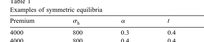
We can illustrate our results by selecting plausible values of model parameters. Table 1 shows equilibrium values of the contribution level for different levels of a
and t, holding fixed Ps4000, and shs800. Note that the value shs800 may be interpreted as follows. Consider a firm in a symmetric equilibrium that considers raising its contribution by US$100. Then if shs800, 5% of those workers who have the option to switch to a spouse’s plan will do so. This magnitude of switching is roughly consistent with that reported by Buchmueller
Ž . 15
and Feldstein 1995 . One other check on plausibility is satisfied—the contribu-tion levels in Table 1 have the correct order of magnitude.
Note that very small increases in a can lead to large increases in contribution levels. According to a recent survey by KPMGrHIAA, the fraction of married workers with working spouses has increased from 63% to 71% between 1983 and 1993, and the fraction of workers with working spouses has increased from 38% to
13
In the limit, as t approaches 1, the equilibrium contribution level would approachy`.
14
To see this, suppose that initially Ps3000 and Cs1000. Now let insurance prices double so that
Ž .
Ps6000 and that hP falls by 50%. Under these conditions, the contribution C would double to 2000.
15 Ž .
Table 1
Examples of symmetric equilibria
Premium sh a t Contribution
4000 800 0.3 0.4 200
4000 800 0.4 0.4 1330
4000 800 0.5 0.4 1990
4000 800 0.4 0.35 1850
4000 800 0.4 0.45 730
42%. The numerical examples suggest that even these seemingly small changes can lead to large increases in contributions. As the contribution levels increase with a, it is interesting to note that the aggregate take-home income of families with two working spouses increases. But workers with stay-at-home spouses
Ž
suffer, as they bear the tax burden on the additional contribution. In expectation,
.
of course, all workers are equally well off at all times.
3. Equilibrium with two types of firms
Discussion of employer-sponsored health insurance often points to the disparity between offerings of large and small firms. Small firms apparently face slightly higher premia than do large firms, yet are much less likely to offer insurance. Those that do offer insurance offer somewhat less generous benefits and require
Ž .
40 to 50% larger employee contributions Morrisey et al., 1994 . We use our model of employer competition to show that firms facing slightly higher premia may require substantially higher contributions. This may be broadly interpreted to imply that those firms may offer substantially less attractive insurance.
We use the same notation as before, with the following exceptions. There are two types of firms, subscripted as B and S. We let PS)P . A fractionB l of all firms are of type S. In equilibrium, all firms of a given type require the same contribution, and the contribution maximizes individual firm profits given the contributions required by other firms. Using similar methods to those used to derive the optimal contribution when all firms are identical we obtain the following first order conditions for firms of types S and B: 16
S B
tr
Ž
1yt.
1y0.5alyaŽ
1yl. Ž
H C yC.
S S B
y
Ž
PSyC.
alh 0Ž .
qaŽ
1yl. Ž
h C yC.
s0,Ž
11.
B S
tr
Ž
1yt.
1yalH CŽ
yC.
y0.5aŽ
1yl.
B B S
y
Ž
PByC.
alh CŽ
yC.
qaŽ
1yl. Ž .
h 0 s0.Ž
12.
16
In Appendix A, we compute the following comparative static results:
S B
EC
Ž
1yt.
ylt EC ylts ; s .
EPS PsP 1y2 t EPS PsP 1y2 t
S B S B
We conclude that when PS is close to PB and t-0.5, then an increase in the premium for the small firm will increase the equilibrium contribution of the small firm and decrease the equilibrium contribution of the large firm. Furthermore, combining these expressions, we easily find that
S B
E
Ž
C yC.
1yts ,
EPS PsP 1y2 t
S B
so the difference in the contribution levels changes by more than the difference in the premiums.
3.1. More numerical examples and an intuition
[image:11.595.63.345.46.96.2]As before, we illustrate this key finding by computing equilibria using plausible parameter values. Table 2 presents these equilibria. The first three rows of the table show equilibria as small firms face slightly higher premia than big firms. Consistent with the formal model, the difference between the contributions required of big and small firms exceeds the difference between the premia. The next to last row suggest that the magnitude of this effect is dampened somewhat when a larger percentage of workers work at large firms. This may be because large firms believe there is a greater chance that their employees will be willing to
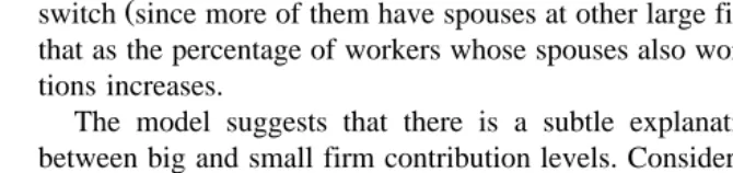
Ž .
switch since more of them have spouses at other large firms . The last row shows that as the percentage of workers whose spouses also work increases, all contribu-tions increases.
The model suggests that there is a subtle explanation for the large wedge between big and small firm contribution levels. Consider the situation where both type B and type S firms face the same premium and require the same contribution.
Ž .
If P increases, then PS SyC increases. From Eq. 11 , type S firms now have an
Table 2
Examples of asymmetric equilibria
Premium Premium sh l a t Contribution Contribution
Ž .S Ž .B Ž .S Ž .B
4000 4000 800 0.5 0.4 0.4 1330 1330
4100 4000 800 0.5 0.4 0.4 1430 1120
4200 4000 800 0.5 0.5 0.4 1300 640
4100 4000 800 0.4 0.4 0.4 1450 1220
[image:11.595.48.383.474.553.2]incentive to raise C. This has the effect of increasing the percentage of workers preferring to purchase insurance from type B firms. More significantly, it implies that the percentage of the big firm’s workers who are indifferent between purchasing from the big and small firms decreases. From the perspective of a big firm, this implies that a smaller percentage of workers will switch to the small firm’s policy if it raises its own contribution. Thus, it prefers to lower its desired contribution to take advantage of the tax break. This drives a wedge between the contributions required by the big and small firms.
3.2. Welfare implications
In our model, total firm output and total labor input do not change as contributions change. Thus, the only welfare changes will derive from changes in insurance purchases. Since we have assumed that the value of insurance always exceeds the cost, distortions do not arise from changes in the quantity of insurance purchased. Rather, welfare changes result if different firms face different insurance costs, the cost differences reflect transactions cost of no value to consumers, and there is a change in the firm from which insurance is obtained
Consider a household in which one spouse works for a type B firm and the other works for a type S firm. Then it is socially optimal for this couple to purchase insurance from the type S firm if and only if their combined idiosyncratic benefit from S’s insurance exceeds the combined idiosyncratic benefit of B’s insurance by at least PSyP . The same logic applies in reverse for purchases ofB B’s insurance. The couple is sure to make the optimal decision if and only if PByCBsPSyC . As we have shown, we would expect PS ByCB-PSyC .S This implies that the couple will make too many purchases of B’s insurance.
We have shown that the interactions between type B and type S firms cause the latter to require excessive contributions relative to the former, thereby distorting insurance purchases. It might therefore be welfare enhancing to subsidize pur-chases of health insurance by small firms, which tend to face higher premia. Interestingly, this could drive up insurance costs, as currently premium differen-tials cause too many individuals to purchase the low cost plans offered by type B
Ž .
firms. The cost increases are offset by increased idiosyncratic benefits.
4. Evidence
equally divided between four strata defined by the number of employees at the establishment: 1–4, 5–9, 10–24, and G25 employees. The overall response rate to the survey was 71%. Response rates varied by state from 59% in New York to 80% in North Dakota. The overall sample size is 22,347 establishments. Cantor et
Ž .
al. 1995 provide additional information on the survey design and content. As a group, these states have demographic characteristics that are generally similar to the characteristics of the entire United States. In particular, Cantor et al.
Ž1995 report that the ten states together have similar health spending per capita,.
percent uninsured, unemployment rates, earnings, and distribution of workers by industry as the entire country.
For each employer, the survey asked the total premium of each plan offered, as well as for both single and family coverage options. Some employers reported a composite premium, and single and family premia were imputed from this value. The premium data we use were also adjusted by the original investigators for
Ž . 17
variations in administrative costs see Cantor et al., 1995 . In addition to
Ž .
premiums, the survey asked the share percentage of the premium that employees were required to pay to purchase the plan. Separate shares were obtained for single and family coverage, where applicable. Using this information, we computed the dollar contribution required of employees to buy single coverage and family coverage for each plan. We then used data on the number of employees enrolled in each plan to compute the average employee share and average employee dollar contribution across all of the plans offered by each employer.
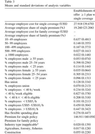
Of the original 22,347 establishments surveyed, 15,591 offered at least one plan with single coverage, and 15,333 offered at least one plan with family coverage. We focus on employers with at least 10 employees. 9581 establishments with more than 10 employees offered a plan with single coverage, and 9509 establish-ments with more than 10 employees offered a plan with family coverage. Excluding employers with missing data for one or more of the explanatory variables left 8716 establishments with single plans and 8648 establishments with family plans. Table 3 summarizes the characteristics of the two samples.
We examine four regressions. The first two examine individual health insurance policies; the second two examine family policies. Our model is cast in terms of family policies, however, many of the issues that we raise could also apply to individual plans. For example, the employer might require a large contribution towards an individual plan so as to discourage employees from obtaining individ-ual policies to complement their spouses’ family coverage. Alternatively, employ-ers of young workemploy-ers may require contributions towards individual plans so as to encourage their employees to obtain coverage through their parents’ plans. While
17
Table 3
Means and standard deviations of analysis variables
Establishments that Establishments that offerG1 plan with offerG1 plan with single coverage family coverage
Ž . Ž .
Average employee cost for single coverage US$ 27.918 39.670 –
Ž . Ž .
Average employee share of single premium % 19.260 23.206 –
Ž . Ž .
Average employee cost for family coverage US$ – 155.043 129.507
Ž . Ž .
Average employee share of family premium % – 41.873 30.689
Ž . Ž .
10–49 employees 0.637 0.481 0.635 0.482
Ž . Ž .
50–99 employees 0.148 0.355 0.148 0.355
Ž . Ž .
100–499 employees 0.167 0.373 0.168 0.374
Ž . Ž .
500–999 employees 0.027 0.161 0.027 0.161
Ž . Ž .
G1000 employees 0.022 0.148 0.022 0.148
Ž . Ž .
% employees maleG55 years 0.053 0.074 0.053 0.074
Ž . Ž .
% employees male 25–54 years 0.398 0.256 0.399 0.256
Ž . Ž .
% employees male-25 years 0.114 0.144 0.114 0.144
Ž . Ž .
% employees femaleG55 years 0.035 0.064 0.035 0.064
Ž . Ž .
% employees female 25–54 years 0.305 0.231 0.305 0.231
Ž . Ž .
% employees female-25 years 0.096 0.131 0.096 0.130
Ž . Ž .
Has union 0.128 0.334 0.129 0.335
Ž . Ž .
% employees union 0.070 0.213 0.071 0.214
Ž . Ž .
% employees-40 hrweek 0.234 0.324 0.232 0.324
Ž . Ž .
-40 hrweek eligible 0.827 0.378 0.828 0.377
Ž . Ž .
%-40 h= -40 h eligible 0.208 0.318 0.207 0.317
Ž . Ž .
% employees-US$5rh 0.101 0.211 0.101 0.210
Ž . Ž .
% employees US$5–US$10rh 0.450 0.304 0.450 0.304
Ž . Ž .
% employees)US$10rh 0.447 0.342 0.448 0.342
Ž . Ž .
Has flexible spending plan 0.276 0.447 0.277 0.448
Ž .
Premium for single policy 146.911 60.058 –
Ž .
Premium for family policy – 379.383 127.873
a Ž . Ž .
Industry type inapplicable 0.020 0.139 0.020 0.140
Ž . Ž .
Agriculture, forestry, fisheries 0.017 0.128 0.016 0.127
Ž . Ž .
Construction 0.055 0.228 0.055 0.228
Ž . Ž .
Mining and manufacturing 0.176 0.381 0.176 0.381
Ž . Ž .
Transportation, communications, public utility 0.061 0.240 0.062 0.241
Ž . Ž .
Wholesale trade 0.089 0.285 0.090 0.286
Ž . Ž .
Retail trade 0.190 0.392 0.189 0.392
Ž . Ž .
Finance, insurance, real estate 0.138 0.345 0.139 0.346
Ž . Ž .
Professional services 0.209 0.407 0.209 0.406
Ž . Ž .
Other services 0.045 0.207 0.044 0.206
Ž . Ž .
Colorado 0.094 0.292 0.094 0.292
Ž . Ž .
Vermont 0.098 0.297 0.098 0.297
Ž . Ž .
New York 0.108 0.310 0.108 0.310
Ž . Ž .
Oregon 0.105 0.306 0.104 0.306
Ž . Ž .
Florida 0.094 0.292 0.094 0.291
Ž . Ž .
New Mexico 0.098 0.297 0.098 0.297
Ž . Ž .
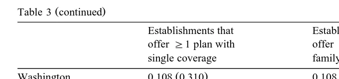
Ž .
Table 3 continued
Establishments that Establishments that offerG1 plan with offerG1 plan with
single coverage family coverage
Ž . Ž .
Washington 0.108 0.310 0.108 0.310
Ž . Ž .
Oklahoma 0.092 0.289 0.092 0.290
Ž . Ž .
Minnesota 0.105 0.306 0.104 0.306
N 8716 8648
a
Public employers and establishments with)5000 employees were coded as ‘inapplicable’ for type of industry on the survey.
we do not explicitly model such situations, we suspect that these incentives, though present, are not as strong as those regarding family plans.
We examine two dependent variables for both independent and family policies: the nominal employee contribution and the employee contribution as a percentage of the total premium. The latter may be more appropriate, for the following reason. In our model, insurance plans offer identical benefits, but larger firms pay less than do smaller firms. Our model predicts that employees of larger firms will make smaller contributions towards any given plan. But, in the data, larger firms tend to offer more generous plans than do smaller firms. For this reason alone they might be expected to require larger contributions. Thus, the net effect of firm size on the nominal level of contributions is indeterminate. However, the model suggests that employees in larger firms should pay lower contributions as a percentage of total premiums.
We examine several predictors other than firm size. A key variable in our model is the percentage of workers with working spouses. We do not have a direct measure of this. Based on labor market participation, we posit that working women are more likely to have working spouses than are working men, especially men over 55 years old. Hence, we predict that firms with a high percentage of female employees will have higher contributions, ceteris paribus, and that firms with a high percentage of male employees over 55 years old will have lower contributions, ceteris paribus.
It is generally accepted that insurance costs are higher at firms that have a high percentage of part time workers covered by insurance. We predict, therefore, that such firms will have higher contributions. We also control for union status, the wage distribution at each firm, and whether the firm offers flexible spending accounts. Lastly, we include premiums. The premium may reflect unmeasured plan quality and so may be endogenous. Excluding premiums does not change our remaining results.
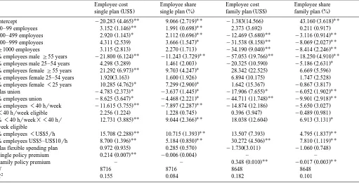
contri-() D. Drano Õ e et al. r Journal of Health Economics 19 2000 121 – 140 Table 4 Regression results
Employee cost Employee share Employee cost Employee share
Ž . Ž . Ž . Ž .
single plan US$ single plan % family plan US$ family plan %
UU UU UU
Ž . Ž . Ž . Ž .
Intercept y20.283 4.465 9.066 2.719 y1.383 14.566 43.160 3.618
UU UU
Ž . Ž . Ž . Ž .
50–99 employees 3.152 1.146 1.991 0.698 2.373 3.692 0.211 0.917
U UU UU UU
Ž . Ž . Ž . Ž .
100–499 employees 2.920 1.143 2.112 0.696 y12.469 3.680 y3.116 0.914
U UU UU
Ž . Ž . Ž . Ž .
500–999 employees 4.311 2.539 3.666 1.547 y31.538 8.158 y8.069 2.027
UU UU
Ž . Ž . Ž . Ž .
G1000 employees 3.115 2.813 2.270 1.713 y34.190 9.040 y8.414 2.246
UU UU UU UU
Ž . Ž . Ž . Ž .
% employees maleG55 years y21.800 6.124 y11.243 3.729 y57.053 19.766 y18.250 4.910
U
Ž . Ž . Ž . Ž .
% employees male 25–54 years 4.298 3.289 1.461 2.003 y20.325 10.590 y5.186 2.631
UU U
Ž . Ž . Ž . Ž .
% employees femaleG55 years 21.292 6.973 9.703 4.247 28.342 22.525 6.669 5.596
Ž . Ž . Ž . Ž .
% employees female 25–54 years 1.920 3.163 1.600 1.926 6.894 10.175 1.747 2.528
Ž .U Ž .U Ž . Ž .
% employees female-25 years 10.285 4.762 7.299 2.900 1.642 15.367 y0.867 3.817
U U U UU
Ž . Ž . Ž . Ž .
Has union y4.783 2.373 y3.637 1.445 y17.906 7.655 y6.052 1.902
U U UU UU
Ž . Ž . Ž . Ž .
% employees union y8.625 3.647 y4.468 2.221 y44.711 11.748 y9.901 2.918
UU UU
Ž . Ž . Ž . Ž .
% employees-40 hrweek y11.615 3.755 y7.897 2.287 y14.874 12.186 y5.650 3.027
Ž . Ž . Ž . Ž .
-40 hrweek eligible 2.256 1.224 1.228 0.745 0.396 3.947 y0.489 0.981
UU UU U
Ž . Ž . Ž . Ž .
%-40 hrweek= -40 hr 12.731 3.885 9.044 2.366 18.038 12.604 6.913 3.131
week eligible
UU UU UU
Ž . Ž . Ž . Ž .
% employees-US$5rh 15.708 2.288 10.715 1.393 13.507 7.393 4.795 1.837
UU UU UU UU
Ž . Ž . Ž . Ž .
% employees US$5–US$10rh 8.700 1.396 5.184 0.850 30.272 4.506 7.810 1.119
Ž . Ž . Ž . Ž .
Has flexible spending plan 0.972 0.935 0.285 0.570 y1.730 3.011 y1.060 0.748
UU
Ž . Ž .
Single policy premium 0.214 0.007 y0.006 0.004 – –
UU UU
Ž . Ž .
Family policy premium – – 0.348 0.010 y0.017 0.003
N 8716 8716 8648 8648
2
R 0.155 0.084 0.182 0.101
Note: Standard errors in parentheses. Models also contain nine SIC code dummies and nine state dummies. U
0.01Fp-0.05. UU
butions than do smaller firms, especially when measured in percentage terms.18 Thus, workers at the smallest firms contribute 8.5% more of the premium cost than do workers at the largest firms. Thus, if the premium is US$4000, the workers at large firms would make US$340 lower contributions. This is consistent with our simulations, where the difference in contributions range from around US$200 to US$700.
Firms with more female workers have higher contributions, and firms with more male workers over age 55 have lower contributions. For example, a one
Ž .
standard deviation 0.05 increase in the percentage of male workers over age 55 is associated with a 1 percentage point reduction in contributions, or US$40 for a US$4000 policy. If we make the unrealistic assumption that all male workers over age 55 have nonworking spouses, and that all other workers have working spouses, then our simulation in Table 1 suggests that a 0.05 increase in the percentage of male workers over age 55 would cause contributions to decrease by US$300 to US$400. Given more reasonable assumptions, the simulation would generate much smaller decreases in contributions, perhaps in line with the empirical estimates.
Lastly we find that firms with more covered part time workers have higher
Ž .
contributions. A one standard deviation increase 0.32 is associated with a 22 percentage point increase in contributions, or US$880 for a US$4000 policy. This is not out of line with our simulations in Table 2, provided that part time workers are more costly to insure.
5. Discussion
The lay view is that employers raise contributions when ‘insurance becomes too costly.’ In an important sense this is consistent with our model. Firms would like their employees to have insurance. But they would prefer it if they obtained their insurance through their spouse’s employer, especially as the price of insurance increases. We have analyzed the competitive interaction between firms as they trade off the tax benefits of generous insurance coverage against the direct savings from shifting coverage onto spouses. The outcome of this interaction is highly sensitive to a number of parameters, including tax rates, spousal work decisions, and interfirm differences in premia.
The predictions of our model are consistent with observed patterns in the cross-section. As predicted by the model, firms that have higher costs of insurance tend to have disproportionately higher contributions. Firms whose employees are less likely to have working spouses have lower contributions, which is also consistent with our model.
18 Ž .
Although we develop the model in terms of premia and contribution levels for a given insurance plan, our findings may generalize to the choice of plan and decision to offer a plan. For example, our findings suggest that if small firms face slightly higher premia, they may disproportionately offer poor or no insurance benefits as a way to encourage workers to select their spouse’s employer’s plan.
Ž .
This is consistent with the findings of Morrisey et al. 1994 and Cantor et al.
Ž1995 that show that small firms offer less generous insurance than do large. Ž .
firms, and the finding of Liebowitz and Chernew 1992 that states small premia differentials may cause a large percentage of small firms to drop coverage.
Our model also identifies several factors that may have contributed towards the rapid increase in contributions over the past two decades. Our model suggests that contributions should increase when:
1. The price of insurance is high relative to the idiosyncratic differences in taste for insurance;
2. The tax rate is low; and
3. The fraction of workers with working spouses is high
Ž .
The sharp rise in insurance premia during the past two decades suggest that 1 is more likely to hold today than during the 1970s. At the same time, the marginal income tax rate is lower than during the 1970s.19 Finally, the fraction of workers with working spouses has steadily risen.20All of these trends are consistent with rising contribution.
Acknowledgements
We thank Howard Bolnick for his helpful comments regarding tax treatment of health insurance, and James Dana for computing numerical examples. Richard Frank, David Cutler, Michael Chernew and Jon Gruber made valuable sugges-tions.
Appendix A
Ž
Proof of Lemma 1: First note that the individual rationality constraint
in-Ž ..
equality 4 must bind at the optimum; if not, the optimal strategy would be to make the wage as small as possible and the contribution as large as possible. We
19 Ž .
Long and Scott 1984 discuss how the 1981 Tax Act reduced marginal tax rates and was expected to decrease demand for nontaxed employee fringe benefits.
20 Ž .
For example, data from the U.S. Department of Commerce 1996 suggest that in 1980, 56% of
Ž .
Ž .
substitute in for the base wage from 4 into the objective function and see that the firm solves the following program:
U U U
Min W q 1r
Ž
1yt. Ž
1ya. Ž
CyC.
ya GŽ Ž
C,C.
4C
U U U
yG
Ž
C ,C.
qŽ
PyC.
1yaH CŽ
yC.
s.t. and CG0.
Differentiating the objective function with respect to C gives us the following condition:
X U U
1ya r 1yt y ar 1yt G C,C y 1yaH CyC
Ž
. Ž
.
Ž
.
Ž
.
Ž
Ž
.
.
y
Ž
PyC.
ah CŽ
yCU.
s0.Ž .
5 We assume that the second derivative of the objective function is positive, so the first order condition is necessary and sufficient for an optimum so long as C is, inX
Ž U. Ž Ž U.. Ž .
fact, non-negative. Noting that G C,C s 1yH CyC , Eq. 5 can be rewritten as the expression given in the Lemma.I
( ) ( )
A.1. Computation of comparatiÕe statics of Eqs. 11 and 12
1Ž S B .
Defining this set of equations as F C ,C ; P , P ,S B l,a,t s0 and
2Ž S B . SŽ .
F C ,C ; P , P ,S B l,a,t s0, an implicit solution, C P , P ,S B l,a,t and
BŽ .
C P , P ,S B l,a,t , exists if and only if the Jacobian matrix is non-singular. It is straightforward to verify that this condition holds when PSsP , for in this caseB
S B Ž . XŽ B S.
C sC as in the previous section , h C yC s0, and many of the terms simplify.
1 1
EF EF
S B
EC EC
Js 2 2
EF EF
S B
EC EC PSsPB
t t
ah 0
Ž .
1yŽ
1yl.
ž /
ah 0Ž . Ž
1yl.
ž /
1yt 1yt
s
t t
ah 0
Ž .
lž /
ah 0Ž .
1ylž /
1yt 1yt
Ž . w Ž .x2wŽ . Ž .x
SŽ . identify the partial derivatives of the implicit functions C P , P ,S B l,a,t and
BŽ .
C P , P ,S B l,a,t evaluated at PSsP :B
S 1
EC yEF
EPS y1 EPS
sJ
B 2
EC yEF
EPS EPS
PSsPB PSsPB
t t
1yl
ž /
yŽ
1yl.
ž /
ah 0
Ž .
1yt 1yt ah 0Ž .
s
t t
Det J
Ž .
PSsPB 0yl
ž /
1yŽ
1yl.
ž /
1yt 1yt
which reduces to:
S B
EC
Ž
1yt.
ylt EC ylts ; s .
EPS PsP 1y2 t EPS PsP 1y2 t
S B S B
References
Buchmueller, T., Feldstein, P., 1995. The effect of price on switching among health plans. U.C. Irvine, unpublished manuscript.
Cantor, J.C., Stephen, L., Marquis, M.S., 1995. Private employment-based health insurance in ten
Ž .
states. Health Affairs 14 2 , 199–211.
Employee Benefit Retirement Institute, 1995. EBRI Databook on Employee Benefits, 3rd edn. Washington, DC.
Lazear, E., 1995. Personnel Economics. MIT Press, Cambridge, MA.
Levy, H., 1998. Who pays for health insurance? Employee contributions to health insurance premiums. U.C. Berkeley, unpublished manuscript.
Liebowitz, A., Chernew, M., 1992. The firm’s demand for health insurance in health benefits and the workplace. U.S. Department of Labor, Washington, DC.
Long, J., Scott, F., 1984. The impact of the 1981 tax act on fringe benefits and federal tax revenues. National Tax Journal 37, 185–194.
Morrisey, M., Jensen, G., Morlock, R., 1994. Small employers and the health insurance market. Health
Ž .
Affairs 13 5 , 149–161.
Scott, F., Berger, M., Black, D., 1989. Effects of tax treatment of fringe benefits on labor market segmentation. Industrial and Labor Relations Review 42, 216–229.