Drawing Undirected Graphs
TimGA: Un Algoritmo Gen´
etico para Dibujar Grafos no
Dirigidos
Timo Eloranta (
@
)
Erkki M¨akinen (
)
Department of Computer and Information Sciences, P.O. Box 607, FIN-33014 University of Tampere, Finland
Abstract
The problem of drawing graphs nicely contains several computa-tionally intractable subproblems. Hence, it is natural to apply genetic algorithms to graph drawing. This paper introduces a genetic algorithm (TimGA) which nicely draws undirected graphs of moderate size. The aesthetic criteria used are the number of edge crossings, even distri-bution of nodes, and edge length deviation. Although TimGA usually works well, there are some unsolved problems related to the genetic crossover operation of graphs. Namely, our tests indicate that TimGA’s search is mainly guided by the mutation operations.
Key words and phrases: Genetic algorithm, graph drawing, undi-rected graphs.
Resumen
El problem de dibujar grafos apropiadamente contiene varios sub-problemas computacionalmente intratables. Por lo tanto es natural aplicar algoritmos gen´eticos al dibujo de grafos. Este art´ıculo introdu-ce un algoritmo gen´etico (TimGA) que dibuja bien grafos no dirigidos de tama˜bo moderado. Los criterios est´eticos usados son el n´umero de cruces de aristas, la distribuci´on uniforme de los nodos y la desviaci´on de las longitudes de las aristas. Aunque TimGA usualmente trabaja bien, hay algunos problems no resueltos relacionados con la operaci´on gen´etica de cruzamiento de grafos. De hecho, nuestras pruebas indican
Recibido 2000/12/13. Revisado 2001/09/15. Aceptado 2001/10/10. MSC (2000): Primary 68R10, 05C85.
que la b´usqueda realizada por TimGA est´a guiada principalmente por las operaciones de mutaci´on.
Palabras y frases clave: algoritmo gen´etico, dibujo de grafos, grafos no dirigidos.
1
Introduction
The problem of drawing graphs nicely is completely solved only in some very special cases [8]. Irrespective of the aesthetic criteria used, the problem usually contains several computationally intractable subproblems [2]. This motivates the use of methods of genetic algorithms and other soft-computing approaches. For earlier works following this line of research, see e.g. [4, 6, 10, 12, 13, 14, 16, 17].
This paper introduces a genetic algorithm TimGA (Timo’s Genetic Algo-rithm) for drawing undirected graphs. TimGA owes some of its basic data structures to Groves et al.’s algorithm [10]. However, since undirected edges instead of directed ones are considered, most decisions differ from those made by Groves et al. TimGA outputs grid drawings with straight line edges.
In what follows we assume that the reader is familiar with the basics of genetic algorithms and graph theory as given e.g. in [15] and [11], respectively.
2
Selection and the evaluation function
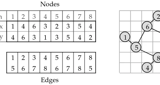
TimGA draws graphs in anN×N matrix. Each node is located in a square of the matrix and all edges are drawn as straight lines. To represent a graph with n nodes and m edges we use a 2×n matrix to indicate the positions of the nodes and a 2×m matrix to indicate the edges by storing pairs of nodes. The corresponding end points are then found from the node matrix. Figure 1 shows a simple example of the representation used. Groves et al. [10] have used similar representation for nodes. It should be noted that while our representation of graphs resembles that in [10], the algorithms otherwise differ a lot. For example, the evaluation fucntion used in [10] is totally different than ours.
One of the crucial points of a genetic algorithm is the method of selecting chromosomes to the genetic operations. TimGA uses thelinear normalization
1
3
4
5
6
7
8
x
y
1
1
2
2
3
3
3
3
4
4
4
4
5
5
6
6
1
8
5
5
6
6
4
7
8
8
5
2
7
7
3
6
Edges
Figure 1: The representation of a sample graph.
(e.g. 100) and the other chromosomes get stepwise decreasing constant values (e.g. 98, 96, 94,...). Chromosomes are then selected to the genetic opera-tions proportionally to the values so obtained. Depending on the length of the step (the difference between the consecutive constant values; two in the above example), this method can be parametrized to give a desired emphasis to the best chromosomes. TimGA allows the user to set the length of the step. By default, TimGA uses elitist selection, i.e., the best chromosome is always chosen as such to the next generation.
The aesthetic criteria used are imported to genetic graph drawing algo-rithms in the form of the evaluation function (also called the fitness function). TimGA tries to minimize the number of edge crossings, to distribute the nodes evenly over the drawing area, and to minimize the deviation of edge lengths.
The positive terms (to be maximized) in the evaluation function are
• Minimum Node Distance Sum: The distance of each node from its near-est neighbour is measured, and the distances are added up. The bigger the sum the more evenly the nodes are usually distributed over the drawing area.
• Minimum Node Distance (Number of Nodes×(Minimum Node Distance)2 ): This term helps in distributing the nodes. The square of minimum node distance is multiplied by the number of nodes.
• Edge Length Deviation: The length of each edge is measured and com-pared to the ”optimal”edge length, which is little more than the mini-mum edge length found from the present layout.
• Edge Crossings: The number of edge crossings is multiplied by the size of the drawing grid. (The grid is always a square.)
The evaluation function is combined from the above variables. The exe-cutions reported in this paper are run with the following default coefficients:
2×Minimum Node Distance Sum
−2×Edge Length Deviation
−21
2×(Edge Length Deviation / Minumum Node Distance) 1
4×(Number of Nodes×(Minimum Node Distance) 2
)
−1×(Edge Crossings×(Grid Size)2 ).
These coefficients were found in our preliminary test runs.
TimGA spends most of its computation time in evaluating the chromo-somes. One of the problematic issues is the counting of the number of edge crossings. There is a well-known method based on cross productions to check whether two line segments intersect [4, pp. 889-890]. More advanced methods are introduced by Bentley and Ottmann [1] and Chazelle and Edelsbrunner [3]. Unfortunately, the method of Chazelle and Edelsbrunner, though asymp-totically time optimal, is too complicated for the present application. On the other hand, the Bentley and Ottman’s algorithm is too slow. Thus, we have to use a method of our own for counting the number of edge crossing. We keep track of the movements of the nodes, and update the number of edge crossings only when a node is moved. This method outperforms the Bentley and Ottman’s algorithm in the present situation.
3
The genetic operations
2 1 4 8 5 7 6 3
Child-2
2 4 5 6 7 8 1 3Child-1
2 5 4 6 7 8 1 3Parent-2
1 2 3 7 4 5 6 8Parent-1
2 1 4 8 5 7 6 3Child-2
2 4 5 6 7 8 1 3Child-1
2 5 4 6 7 8 1 3Parent-2
1 2 3 7 4 5 6 8Parent-1
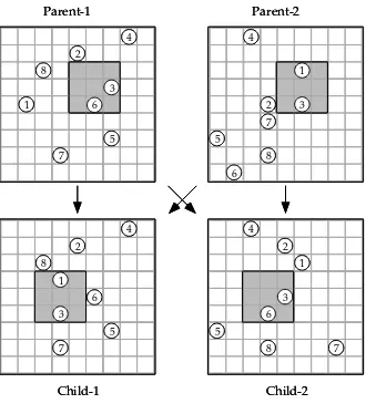
The sample RectCrossover operation of Figure 2 uses rectangles of size 3×3; these are painted grey in the figure. (Other sizes of rectangles were also used in our preliminary tests, but 3×3 seems to be the optimal rectangle size.) The parents change the positions of the nodes 3 and 6 (from Parent-1) and nodes 1 and 3 (form Parent-2). The nodes 1 and 3 keep their relative positions in the grey area when it is moved from Parent-2 to Child-1. Moreover, since the chosen rectangle in Child-1 is empty, the rest of the nodes in Child-1 can keep their old positions, i.e. the positions they have in Parent-1. On the other hand, in Child-2 there are two nodes in the chosen 3×3 rectangle (nodes 2 and 7). These must be moved outside the area. The first possible place is the square where the corresponding node is in the other parent. Since node 2 of Parent-1 is in the square (2,5), this is the new position of the node in Child-2. This method does not work with node 7, since the square (8,4) is already occupied by node 8. So, we have to place node 7 to an randomly chosen free square (8,8). RectCrossover closely resembles the Cont-Crossover operation of [9].
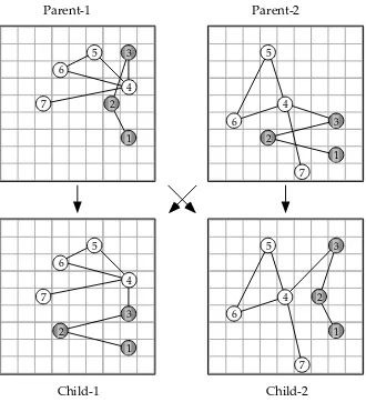
The other crossover operation in TimGA is called ThreeNodeCrossover. A connected subgraph consisting of three nodes is chosen. The parents then exchange the positions of the three nodes in question. If some of the new positions are already occupied, the nodes in question are kept unchanged. A sample ThreeNodeCrossover is shown in Figure 3.
Groves et al. [10] introduced about a dozen different mutation operations. In our tests we have used 16 different mutations of which 11 are from [10] and the five rest are new. Our tests indicate that mutation operations applied to edges usually have better performance than those applied to nodes. The following eight mutation operations performed best in our tests:
• SingleMutate: Choose a random node and move it to a random empty square [10].
• SmallMutate: Choose randomly two squares from the drawing area such that at least one of them contains a node. If both contain a node, exchange the nodes. If only one of them contains a node, then move the node from the present location to the empty square [10].
• LargeContMutate: Choose two areas of equal size and shape from the grid. Exchange the contents of the chosen areas [10].
1 2
3 5
4 6
7
Child-2
74 5 6
2
1 3
Child-1
5
4 6
7 2
1 3
Parent-2
1 7
4 5 6
[image:7.595.174.504.245.616.2]2 3
Parent-1
• EdgeMutation-2: Like EdgeMutation-1, but the length and angle of the edge is kept unchanged, if possible.
• TinyEdgeMove: Like EdgeMutation-2, but the edge is moved only at most one square both horizontally and vertically.
• TwoEdgeMutation: Like EdgeMutation-2, but two edges incident with a same node are moved.
• TinyMutate: Like SingleMutate, but the node is moved only at most one square both horizontally and vertically.
The probability of using a certain mutation type depends on its perfor-mance in our tests. The operations introduced above have the following rel-ative probabilities (the bigger the probability the better performance in our tests):
TwoEdgeMutation 12/65 EdgeMuation-2 10/65 SingleMutate 10/65 EdgeMutation-1 5/65 LargeContMutate 5/65 SmallMutate 5/65 TinyMoveEdge 5/65 TinyMutate 5/65.
Moreover, eight additional mutation operations introduced in [10] are used with relative probability 1/65. Note that the mutation operations clearly have different roles: some of them are more suitable for tentative searching and some others for fine tuning.
4
Parameters
This chapter deals with the test runs which were done to fix the various parameters of TimGA. We did over 4000 runs using mainly the following test graphs:
• a cycle with 48 edges
• a triangular grid with 28 nodes and 63 edges
used, the results can be generalized also to other graphs of approximately the same size.
The size of the grid. What is the optimal size of the drawing area for our test graphs? This was tested for grids from 10×10 to 70×70. The optimum size was 40×40, and this size was used in all the tests to be reported. There were only small differences between all the grid sizes from 20×20 to 70×70; grids smaller than 10×10 were clearly inferior (for obvious reasons).
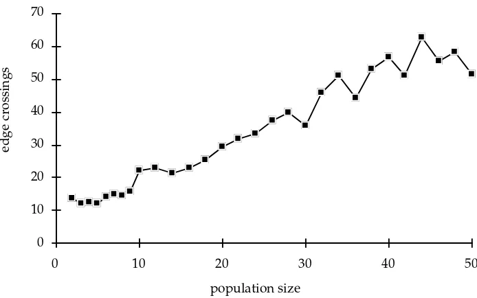
The size of population. Population size should be large enough to give an unbiased view of the search space. On the other hand, too large population size makes the algorithm inefficient, if not intractable. Surprisingly, TimGA seems to works best with very small populations. Figure 4 shows the average numbers of edge crossings with different population sizes after the running time of 15 seconds on a Power Macintosh with our complete tree test graph. (All the tests were executed on a 100 MHz Power Macintosh.) The results with bigger populations were not considerably better even when somewhat longer execution times were allowed.
These results suggest that the population size should not exceed 10. We use the population size 10 in the rest of our tests. Such a small population size might not fit the Schema Theorem, the Building Block Hypothesis [15], and other theoretical principles of genetic algorithms. However small populations give us the best results! We interpret this phenomenon so that the crossover operations used are unable to sift the good properties (called schemata in [15]) of the chromosomes from parents to children, and the search is mainly guided by the mutation operations.
Selection. Our tests advice to use large steps in the linear normalization. This means that the best chromosomes are strongly favoured. This can be considered as a further evidence for the fact that our crossover operations do not help. (Michalewicz [15, p. 57] has noted that the use of selection methods neglecting the actual relative differences between the fitness of chromes is also against the theoretical basis of genetic algorithms. The linear normalization is one of these methods.)
population size 0
10 20 30 40 50 60 70
0 10 20 30 40 50
[image:10.595.166.513.315.532.2]edge crossings
(a)
(b)
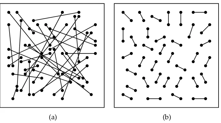
Figure 5: A sample input and the corresponding output.
5
Example layouts
In this chapter we present the results of applying TimGA to some typical graphs. All the drawings (and their computation times) reported in this chapter are produced on a Power Macintosh. The computation times given in this chapter are not averaged over several runs as was done in the results reported in the previous chapters. This means that randomly selected initial populations may distort the results.
Our first example demonstrates the aesthetic criteria used. In Figure 5(a) a set of separate edges is shown. From this input TimGA outputs the drawing shown in Figure 5(b). There are no edge crossings, the edges are distributed evenly over the drawing area, and the edges are of about the same length. The drawing of Figure 5(b) was created in 20 seconds; eliminating all the edge crossings took about a second.
Figure 6 shows how TimGA tends to draw a cycle. This figure indicates that although the evaluation fuction does not contain a valiable directly mea-suring the existence of symmetry in the resulting drawing, the combination of maximizingMinimum Node Distanceand maximizingEdge Length Deviation
Figure 6: An output for a cycle.
(a)
(b)
[image:12.595.193.479.482.637.2](a)
(b)
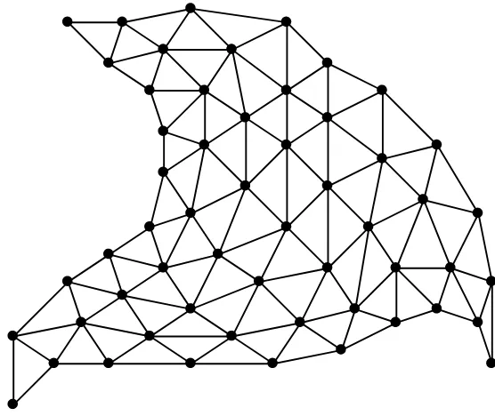
[image:13.595.196.485.289.558.2](c)
Figure 9: A layout for a triangular grid graph.
Figure 7 demonstrates the effect of the grid size. The same graph (the cubic graph) is drawn using the grid sizes 12×12 (Figure 7(a)) and 20×20 (Figure 7(b)). The Figure 7(b) suffers from the tendency of drawing graphs with edges of equal length. This tendency is more easily realized in a grid with more squares.
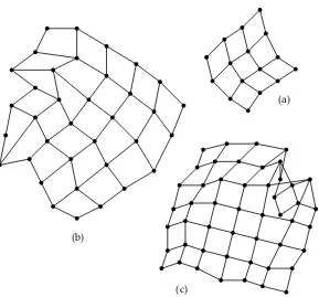
Figure 8 shows three drawings for square grid graphs of different sizes. The graph of Figure 8(a) is drawn in a drawing area of size 22×22, while the other two are drawn in a drawing area of size 40×40. Figure 8(a) was produced in 8 seconds using less than 5000 generations. Figure 8(b) took almost 90 seconds although the result is not completely symmetric. Even worse is the situation with Figure 8(c): after the running time of 10 minutes TimGA was still unable to find a planar drawing. The evaluation function does not ”understand”that moving the top right node of the grid graph upwards would only temporarily cause more edge crossings.
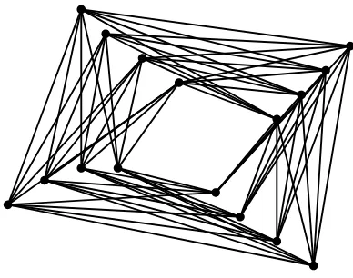
Figure 10: A layout forK8,8
and 135 edges. The computation time was about three and a half minutes (5400 generations).
We end this chapter with some remarks concerning the Edge Crossing Problem (ECP). Given an undirected graphG, ECP is the problem of deter-mining the minimum number of edge crossings (denoted byν(G)) among the layouts of G. ECP is known to be NP-complete [9]. The following approxi-mation is known for the crossing number of complete bipartite graphs [10, p. 123]
ν(Km,n)≤ ⌊m 2 ⌋⌊
m−1 2 ⌋⌊
n
2⌋⌊ n−1
2 ⌋.
TimGA easily reaches the above bound for graphs Km,m, where m ≤ 12. Figure 10 shows a drawing forK8,8.
6
Conclusions
References
[1] Bentley, J. L., Ottmann, T. A. Algorithms for reporting and counting geometric intersections, IEEE Transactions on Computers,C-28(1979) 643–647.
[2] Brandenburg, F. J.Nice drawings of graphs and trees are computationally hard, Tech. report MIP-8820, Fakult f¨ur Mathematik und Informatik, Univ. Passau (1988).
[3] Chazelle, B., Edelsbrunner, H.An optimal algorithm for intersecting line segments in the plane, Journal of the ACM,39(1992) 1–54.
[4] Cimikowski, R., Shope, P.A neural network algorithm for a graph layout problem, IEEE Transactions on Neural Networks, 7(1996), 341–349. [5] Cormen, T. H., Leiserson, C. E. Rivest, R. L.,Introduction to Algorithms.
The MIT Press, 1990.
[6] Davidson, R., Harel, D.Drawing graphs nicely using simulated annealing
, ACM Transactions on Graphics,15(1996) 301–331.
[7] Davis, L. A genetic algorithms tutorial. In L. Davis (ed.), Handbook of Genetic Algorithms. Van Nostrand Reinhold, 1991, 1–101.
[8] G. Di Battista, P. Eades, R. Tamassia and I. G. Tollis, Annotated bibli-ography on graph drawing algorithms,Computational Geometry. Theory and Applications4(1994) 235–282.
[9] M. R. Garey and D. S. Johnson, Crossing number is NP-complete,SIAM Journal of Algebraic Discrete Methods4(1983) 312–316.
[10] L. Groves, Z. Michalewicz, P. Elia and C. Janikow, Genetic algorithms for drawing directed graphs, in: Proceedings of the Fifth International Symposium on Methodologies for Intelligent Systems, (Elsevier North-Holland, 1990) 268–276.
[11] F. Harary,Graph Theory. (Addison-Wesley, 1969).
[14] Markus, A. Experiments with genetic algorithms for displaying graphs, in: Proceedings of the 1991 IEEE Workshop on Visual Languages, IEEE Computer Society Press, 1991, 62–67.
[15] Michalewicz, Z.Genetic Algorithms + Data Structures = Evolution Pro-grams, Springer, 1992.
[16] Rosete-Su´arez,A., Ochoa-Rodr´ıguez, A., Sebag, M. Automatic graph drawing and stochastic hill climbing, in: Proceedings of the Genetic and Evolutionary Computation Conference, vol. 2, Morgan Kaufmann, 1999, 1699–1706.