Changes in the Distribution of
Earnings Volatility
Shane T. Jensen
Stephen H. Shore
Jensen and Shoreabstract
Recent research has documented a rise in the volatility of individual labor earnings in the United States since 1970. Existing measures of this trend abstract from within- group latent heterogeneity, effectively estimating an increase in average volatility for observable groups. We decompose this average and fi nd no systematic rise in volatility for the vast majority of individuals. Increasing average volatility has been driven almost entirely by rising earnings volatility of those with the most volatile earnings, identifi ed ex ante by large past earnings changes. We characterize dynamics of the volatility distribution with a nonparametric Bayesian stochastic volatility model from Jensen and Shore (2011).
I. Introduction
A large literature uses survey data to argue that labor earnings volatil-ity—the expectation of squared individual earnings changes—has increased substan-tially since the 1970s in the United States.1 These papers typically conclude that
volatil-1. Dynan, Elmendorf, and Sichel (2007) provide an excellent survey of research on this subject in their Table 2, including Gottschalk and Moffi tt (1994); Moffi t and Gottschalk (2011); Daly and Duncan (1997); Dynar-ski and Gruber (1997); Cameron and Tracy (1998); Haider (2001); Hyslop (2001); Gottschalk and Moffi tt (2002); Batchelder (2003); Hacker (2006); Comin and Rabin (2009); Gottschalk and Moffi tt (2006); Hertz (2006); Winship (2007); Bollinger, Gonzalez, and Ziliak (2009); Bania and Leete (2007); Altonji, Smith, and Vidangos (2009); Sabelhaus and Song (2010); DeBacker et al. (2012). See also Shin and Solon (2011).
Shane Jensen is an associate professor at the Wharton School, stjensen@wharton.upenn.edu. Stephen Shore is an associate professor at Georgia State University, sshore@gsu.edu. The authors thank Christopher Carroll, Jon Faust, Robert Moffi tt, and Dylan Small for helpful comments, as well as seminar participants at the University of Pennsylvania Population Studies Center, the Wharton School, Dartmouth College, Cergy- Pontoise University, University of Oslo, University of Toulouse, the 2008 Society of Labor Economists Annual Meeting, the 2008 Seminar on Bayesian Inference in Econometrics and Statistics, the 2008 North American Annual Meeting of the Econometric Society, the 2008 Annual Meeting of the Society for Economic Dynamics, the 2009 Foundation du Risque conference, and the 2009 European Summer Symposium in La-bour Economics. They thank Ankita Srivastava for excellent research assistance. The data used in this article can be obtained beginning January 2016 through December 2019 from Stephen H. Shore, 35 Broad Street, Room 1144, Robinson College of Business, Georgia State University, Atlanta, GA 30303. sshore@gsu.edu.
[Submitted December 2012; accepted April 2014]
ISSN 0022- 166X E- ISSN 1548- 8004 © 2015 by the Board of Regents of the University of Wisconsin System
The Journal of Human Resources 812
ity increased in the 1980s and either remained at this level through 2004 (Gottschalk and Moffi tt 2009) or increased through the early 1990s (Shin and Solon 2011; Dynan, Elmendorf, and Sichel 2012; Ziliak, Hardy, and Bollinger 2011).2 By contrast, research
using U.S. administrative data has typically found that volatility has been constant since the mid- 1980s (Dahl, DeLeire, and Schwabish 2011; Sabelhaus and Song 2009).
Variation in earnings volatility across individuals has also been studied. Most papers on this topic examine heterogeneity based on observables or heterogeneity linked to cross- group differences (for example, comparing men and women, young and old). Cross- group differences in volatility trends are considered as well. For example, Ziliak, Hardy, and Bollinger (2011) fi nd that rising family earnings volatility was driven by increasing volatility for husbands while womens’ earnings volatility fell.3
To date, research on earnings volatility trends has generally ignored latent (within- group) individual heterogeneity, effectively estimating an increase in average volatil-ity, either the average for the population at large or the average for a demographic group.4 Most research on heterogeneity and earnings dynamics trends has considered
cross- group differences for observable groups (for example, gender or age). In this paper, we study latent heterogeneity since volatility levels and trends may not be the same for all individuals with the same demographics. We decompose this increase in the average and fi nd that it is far from representative of the experience of most people: There has been no systematic increase in volatility for the vast majority of individuals. The increase in average volatility has been driven almost entirely by a sharp increase in the earnings volatility of those individuals with the most volatile earnings. Further-more, we fi nd that these individuals with high—and increasing—volatility are more likely to be self- employed and more likely to self- identify as risk- tolerant.
Our key fi nding in PSID survey data—that increased average volatility can be ex-plained by increased volatility among the most volatile—may help to reconcile the divergence of trends in average volatility as measured in survey and administrative sources. The high volatility individuals—whom we fi nd to have increasing volatility in survey data—may be captured differently in administrative data. This minority of individuals may have earnings that they report to be increasingly volatile but that administrative data do not show to be volatile. This volatile group is more likely to be self- employed and risk- tolerant; this is exactly the group for which perceptions of earnings and earning swings may diverge from administrative data.
Our main fi nding is apparent in simple summary statistics from the PSID. For ex-ample, divide the sample into cohorts, comparing the minority who experienced very large absolute earnings changes in the past (for example, four years ago) to those who did not. Because volatility is persistent, those identifi ed ex ante by large past earnings
2. Other research on changes over time has focused on business- cycle variation in volatility, including Guvenen, Ozkan, and Song (2012); Storesletten, Telmer, and Yaron (2004); Shore (2010).
3. Trends in other features of earnings dynamics have also been studied, such as the variance of earnings growth rates (Sabelhaus and Song 2010) and inequality (Debacker et al. 2013). Trends in consumption vola-tility have also been studied (Keys 2008, Gorbachev 2011).
Jensen and Shore 813
changes naturally tend to have more volatile earnings today. The earnings volatility of this ex ante high- volatility group has increased since the 1970s while the earnings volatility of others has remained roughly constant.5 This divergence of sample
mo-ments identifi es our key result.
Obviously, these fi ndings could affect substantially the welfare and policy implica-tions of the rise in average volatility. The individuals with the most volatile earnings— whose volatility we fi nd has increased—may be those with the highest tolerance for risk or the best risk- sharing opportunities. Such risk tolerance is apparent implicitly from their willingness to undertake volatile earnings in the fi rst place; it is apparent explictly from answers to survey questions about hypothetical earnings gambles that indicate higher risk tolerance.
While the basic results can be seen in summary statistics, providing a complete char-acterization of the dynamics of the volatility distribution is a methodological challenge. Such a characterization is necessary in order to separate trends in permanent versus transi-tory shocks and also to identify patterns throughout the volatility distribution. We use a standard model for earnings dynamics that allows earnings to change in response to per-manent and transitory shocks. What is less standard is that we allow the variance of these shocks—our earnings volatility parameters—to be heterogeneous and time- varying in a
fl exible way. Specifi cally, we use the Markovian Hierarchical Dirichlet process (MHDP) prior model developed in Jensen and Shore (2011) that allows the cross- sectional distri-bution of earnings volatility to have a fl exible shape and evolution over time.
In Section II, we discuss our data and the summary statistics that drive our results. In Section III, we present our statistical model including the labor earnings process (Sec-tion IIIA), the structure we place on heterogeneity and dynamics in volatility parameters (Section IIIB), and our estimation strategy (Section IIIC). In Section IV, we show the results obtained by estimating our model on the data. Increases in the average volatility parameter are due to increases in volatility among those with the most volatile earnings (Section IVB). We fi nd that the increase in volatility has been greatest among the self- employed and those who self- identify as risk- tolerant (Section IVE) and that these groups are disproportionately likely to have the most volatile earnings (Section IVD). Increases in risk are present throughout the age distribution, education distribution, and earnings distribution (Section IVE). Section V concludes with a discussion of welfare implications.
II. Data and Summary Statistics
A. Data and Variable Construction
Data are drawn from the core sample of the Panel Study of Income Dynamics (PSID). The PSID was designed as a nationally representative panel of U.S. households. It
The Journal of Human Resources 814
tracked families annually from 1968 to 1997 and in odd- numbered years thereafter; this paper uses data through 2009. The PSID includes data on education, earnings, hours worked, employment status, age, and population weights to capture differential fertility and attrition. In this paper, we limit the analysis to men aged 22 to 60; we use annual labor earnings as the measure of income and subsequently use income volatility and earnings volatility interchangeably.6 Table 1 presents summary statistics from these data.
We want to ensure that changes in earnings are not driven by changes in the top- code (the maximum value for earnings entered that can be entered in the PSID). The lowest top- code for earnings was $99,999 in 1982 ($202,281 in 2005 dollars) after which the top- code rises to $9,999,999. So that top- codes will be standardized in real terms, this minimum top- code is imposed on all years in real terms, so the top- code is $99,999 in 1982 and $202,281 in 2005. Because our earnings process in Section IIIA does not model unemployment explicitly, we need to ensure that results for the log of earnings are not dominated by small changes in the level of earnings near zero (which will imply huge or infi nite changes in the log of earnings). To address this concern, we replace values that are very small or zero with a nontrivial lower bound. We choose as this lower bound the earnings from a half- time job (1,000 hours per year) at the real equivalent of the 2005 federal minimum wage ($5.15 per hour).7 Results are robust
6. Labor earnings in 1968 is labeled v74 for husbands and has a constant defi nition through 1993. From 1994, we use the sum of labor earnings (HDEARN94 in 1994) and the labor part of business income (HDBUSY94), with a constant defi nition through 2009. Note that data are collected on household “heads” and “wives” (where the husband is always the “head” in any couple). We use data for male heads so that men who are not household heads (as would be the case if they lived with their parents) are excluded.
7. This imposes a bottom- code of $5,150 in 2005 and $2,546 in 1982. Note that the difference in log earnings between the top- and bottom- code is constant over time so that differences over time in the prevalence of predictably extreme changes cannot be driven by changes in the possible range of earnings changes. The vast majority of the values below this bound are exactly zero. This bound allows us to exploit transitions into and out of the labor force. At the same time, the bound prevents economically unimportant changes that are small in levels but large and negative in logs from dominating the results.
Table 1
Summary Statistics
Mean
Standard
Deviation Minimum Maximum
Year 1988.2 11.1 1968 2009
Age (years) 39.0 10.3 22 60
Education (years) 12.9 3.1 0 17
Number of observations/person 15.3 8.9 2 34
Married (1 if yes, 0 if no) 0.84 0.36 0 1
Black (1 if yes, 0 if no) 0.06 0.24 0 1
Annual earnings (2005 $) $49,168 $58,526 0 $4,743,650
Annual earnings ($) $31,030 $52,569 0 $5,210,000
Family size 3.2 1.5 1 14
Jensen and Shore 815
to other values for this lower bound, such as the earnings from full- time work (2,000 hours per year) at the 2005 minimum wage (in real terms).8
We model the evolution of “excess” log labor earnings. This is taken as the residual from an equal- weighted regression to predict the natural log of labor earnings (top- and bottom- coded as described). We use as regressors: a cubic in age for each level of educational attainment (none, elementary, junior high, some high school, high school, some college, college, graduate school); the presence and number of infants, young children, and older children in the household; the total number of family members in the household; and dummy variables for each calendar year. Including calendar year dummy variables eliminates the need to convert nominal earnings to real earnings explicitly. Although this step is standard in the earnings process literature, it is not necessary to obtain our results. The results to follow are qualitatively the same and quantitatively similar when we use log earnings in lieu of excess log earnings.
Table 2 presents data on the distribution of real annual earnings in Column 1 (im-posing top- and bottom- code restrictions in parentheses). Although the mean real earn-ings is nearly identical with and without top- and bottom- code restrictions ($49,168 versus $47,502), these restrictions on extreme values reduce the standard deviation of real earnings from $58,526 to $34,607. Column 2 shows the distribution of “excess” log labor earnings. Because excess log earnings is the residual from a regression, its mean is zero.
Column 3 presents the distribution of one- year changes in excess log labor earn-ings. Naturally, the mean of one- year changes is close to zero. The interquartile range of one- year changes is –0.1162 to 0.1475; excess log earnings does not change more than 11.62 to 14.75 percent from year to year for most individuals. However, there are extreme changes so the standard deviation (0.50) is far greater than the interquartile range. This implies either that changes to earnings have fat tails (so that everyone faces a small probability of an extreme change) or, alternatively, that there is hetero-geneity in volatility (so that a few people face a nontrivial probability of an extreme change). Unless a model is identifi ed from parametric assumptions, these are obser-vationally equivalent in a cross- section of earnings changes. However, heterogeneity and fat tails have different implications for the time- series of volatility, and we exploit these in the paper.
B. Volatility Summary Statistics
Table 3 shows the evolution of volatility sample moments over time. The fi rst three columns show the variance of permanent labor earnings changes.9 The fi nal three
pres-8. The Winsorizing strategy employed here is obviously second best to a strategy of modeling a zero earn-ings explicitly. Unfortunately, such a model is not feasible given the complexity added by evolving and heterogeneous volatility parameters. The other alternative would be simply to drop observations with low earnings though we view this approach as much more problematic in our context; it would explicitly rule out the extreme earnings changes that are the subject of this paper.
The Journal of Human Resources 816
ent two- year squared changes in excess log labor earnings, a raw measure of volatility.10
Note that while the mean size of an earnings change (Columns 1 and 4, Table 3) has increased over time, the median (Columns 2 and 5) has not. This divergence can be explained by an increase in the magnitude of large unlikely changes (Columns 3 and 6). Although not framed in this way, these features of the data have been identifi ed in previous research, including Dynan, Elmendorf, and Sichel (2007).
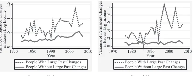
Figure 1 shows the evolution of volatility moments separately for those who are ex ante likely or unlikely to have volatile earnings. The left panel presents the sample mean of the permanent variance; the right panel presents the mean two- year squared excess log earnings change. For each year, the sample is split into two groups (below
10. The fi rst row shows whole- sample results. The second row shows the percent change in the mean, median, or 95th percentile over the sample. This is merely calculated as coeffi cient of an equal- weighted OLS regres-sion of the year- specifi c sample moment on a time trend, multiplied by the number of years (2009 – 1968) and divided by the whole- sample value in the previous row. The coeffi cient and t- statistic from this regression are shown just below. Year- by- year values are then shown.
Table 2
Distribution of Earnings, Excess Log Earnings, and Earnings Changes for Men
Real
Observations 81,470 81,470 59,372 47,173
Minimum $0
25th percentile $25,226 –0.2996 –0.1162 –0.2191
50th percentile $41,178 0.1240 0.0115 0.0576
75th percentile $60,158 0.4628 0.1475 0.3049
95th percentile $111,616 0.9800 0.6995 1.0056
Maximum $4,743,650
($202,381)
2.6541 3.6936 4.0560
Jensen and Shore
817
Table 3
Volatility Sample Moments
Permanent Variance Squared Change
Mean Median 95th Percentile Mean Median 95th Percentile
Average 0.1111 0.0092 0.8530 0.3647 0.0316 2.0735
Percent change 1970–2009 60 –12 100 97 6 125
Slope 0.0016 0.0000 0.0207 0.0086 0.0000 0.0631
(t- statistic) (5.49) (–0.46) (10.94) (10.52) (0.54) (10.48)
1970 — — — 0.1604 0.0213 0.8234
1971 — — — 0.1912 0.0251 0.8700
1972 0.0661 0.0062 0.4118 0.2172 0.0277 1.1290
1973 0.0815 0.0044 0.4763 0.2345 0.0269 1.2375
1974 0.0805 0.0049 0.5097 0.2378 0.0268 1.1527
1975 0.0976 0.0125 0.6321 0.2559 0.0381 1.2749
1976 0.0950 0.0148 0.5849 0.3113 0.0465 1.5665
1977 0.0879 0.0080 0.6961 0.3033 0.0309 1.8656
1978 0.0634 0.0061 0.5674 0.2823 0.0302 1.3542
1979 0.0763 0.0054 0.6424 0.2994 0.0274 1.6838
1980 0.1329 0.0112 0.9286 0.2859 0.0296 1.4833
1981 0.1122 0.0111 0.8734 0.2893 0.0301 1.5687
1982 0.1005 0.0154 0.7534 0.2804 0.0338 1.5905
1983 0.0912 0.0151 0.7114 0.3021 0.0357 1.7242
1984 0.1213 0.0122 0.8770 0.3391 0.0348 1.9942
The Journal of Human Resources
818
Permanent Variance Squared Change
Mean Median 95th Percentile Mean Median 95th Percentile
1985 0.1081 0.0109 0.7951 0.3404 0.0384 1.8061
1986 0.0968 0.0112 0.7054 0.3187 0.0379 1.6570
1987 0.1053 0.0076 0.7975 0.3164 0.0300 1.6815
1988 0.1201 0.0077 0.7888 0.3170 0.0286 1.7579
1989 0.1195 0.0075 0.8355 0.3282 0.0288 1.8451
1990 0.1156 0.0088 0.7773 0.3007 0.0272 1.5713
1991 0.1352 0.0118 1.0330 0.3495 0.0305 1.8224
1992 0.0972 0.0109 0.9209 0.3216 0.0284 1.8102
1993 0.1355 0.0127 1.1158 0.4206 0.0358 2.3956
1994 0.1125 0.0115 0.9153 0.4606 0.0396 2.6854
1995 0.1379 0.0084 1.1266 0.4883 0.0332 3.1723
1996 — — — 0.4744 0.0290 3.0784
1997 0.0870 0.0071 0.8081 0.4549 0.0277 2.8946
1999 0.1242 0.0076 1.0314 0.4514 0.0317 2.9230
2001 0.1195 0.0075 1.1541 0.4493 0.0293 2.9598
2003 0.1416 0.0145 1.2194 0.5924 0.0436 3.6216
2005 0.1523 0.0065 1.2943 0.5944 0.0332 3.6486
2007 0.1303 0.0060 1.1933 0.4464 0.0289 2.7972
2009 — — — 0.4181 0.0259 2.4989
Notes: The year t permanent variance is the product of two- year changes in excess log earnings (from t – 2 to t) and the six- year changes that span them (from t – 4 to t + 2). The year t squared change is from t – 2 to t. The fi rst row shows full sample moments. The second row shows the percent change over the sample, calculated as the coeffi cient of a weighted OLS regression of year- specifi c sample moments on a time trend, multiplied by the number of years (2009–1968) and divided by the full sample moment. The coeffi cient and t- statistic are shown below.
Jensen and Shore 819
median or above 95th percentile) based on the absolute magnitude of permanent (left panel) or squared (right panel) changes four years prior. Unsurprisingly, individuals with large past earnings changes tend to have larger subsequent changes. The tendency to have large changes is persistent so that some individuals have ex ante more volatile earnings than others.
If (as we argue) volatility is increasing for high- volatility individuals but not for low- volatility individuals, then the gap in the sample variance between those with and without large past earnings changes should be increasing over time. This divergence over time in volatility between past low- and high- volatility cohorts is clear in Figure 1. The magnitude of earnings changes has been increasing more for those with large past changes (who are more likely to be inherently high- volatility) than for those without such large past changes (who are not). This is particularly apparent for the permanent variance; for the transitory variance, the fi nding is obscured slightly by the jump in volatility for everyone in the early- to mid- 1990s (when the PSID changed to an automated data collection system, which may have led to increased measurement error in earnings). This divergence illustrates the key stylized fact developed in this paper: The increase in volatility can be attributed to an increase in volatility among those with the most volatile earnings, identifi ed ex ante by large past earnings changes.
Unfortunately, these few sample moments are insuffi cient to provide a rich descrip-tion of the facts on changes in the volatility distribudescrip-tion. First, without a model it is diffi cult to cleanly separate permanent and transitory volatility. Second, any ex ante differences in past volatility do not cleanly separate people by volatility; high levels of past realized volatility may indicate a large shock for a low- volatility individual or a normal- sized shock for a high- volatility individual. A model of earnings dynamics
Figure 1
Comparing Sample Variances for Those With and Without Large Past Earnings Changes
Notes: Following Meghir and Pistaferri (2004), the sample permanent variance is calculated as the product of two- year changes in excess log labor earnings (between years t and t- 2) and the six- year changes that span them (between years t+2 and t- 4). The sample transitory variance is calculated as the square of two- year changes in excess log labor earnings. Individuals are defi ned as low past variances when their sample variance (permanent or transitory, respectively) four years ago is below median; individuals are defi ned as high past variance when their sample variance four years ago is above the 95th percentile. Weighted averages for these groups are presented in each year for which data are available for permanent variance (left panel) and transitory variance (right panel).
The Journal of Human Resources 820
makes this separation possible because it has implications for the frequency with which low- volatility individuals face large shocks. Third, the splitting of the sample based on ex ante realized volatility is necessarily post hoc. For example, the breakdown shown in this paper says nothing about changes in volatility among the least volatile.
III. Statistical Model
A. Earnings Process
Here, we present a standard process for excess log labor earnings for individual i at time
t (following Carroll and Samwick 1997, Meghir and Pistaferri 2004, and many others):
(1) yi,t = pi,t+i,t+ei,t surement error are assumed to be normally distributed with mean zero as well as inde-pendent of one another, over time and across individuals. Permanent earnings are initial earnings (pi,0) plus the weighted sum of past permanent shocks (i,k) with vari-ance ,2i,t ≡ E[
i,t
2]. Transitory earnings are the weighted sum of recent transitory
shocks (i,k) with variance ,2i,t ≡ E[ volatility parameters. These will be allowed to differ between individuals to accom-modate heterogeneity, and to evolve over time. This accomaccom-modates not just an evolv-ing distribution of volatility parameters but also systematic changes over the life cycle in volatility parameters, as suggested by Shin and Solon (2011). “Noise variance” re-fers to the variance of measurement error, 2≡ E[e
i,t 2].11
Permanent shocks come into effect over q periods, and transitory shocks fade com-pletely after q periods.12 As an example of our notation, ,2 denotes the weight placed on a permanent shock from two periods ago, i,t−22, in current excess log earnings; ,2 denotes the weight placed on a transitory shock from two periods ago, i,t−22, in current excess log earnings. While we use the word “shock” for parsimony, these in-novations to earnings may be predictable to the individual, even if they look like shocks in the data. Without loss of generality, we impose the constraint that the weights placed on transitory shocks sum to one (k,k = 1).
11. This measurement error could be subsumed into transitory earnings; it is kept separate only to accom-modate our estimation strategy.
Jensen and Shore 821
B. Heterogeneity and Dynamics
We characterize the dynamics of volatility parameters, i2,t, using a discrete nonpara-metric approach from Jensen and Shore (2011). In such a model, the variable of inter-est— here, the pair i2,t ≡(
,i,t 2 ,
,i,t
2 )—can take one of L possible values (where the
number of these values and the values themselves are estimated from the data). The probability that i2,t takes a given value is a function of (a) the distribution of values in the population, (b) the distribution of values for each individual i, and (c) the number of consecutive years with the most recent value. In other words, i2,t has a given prob-ability of changing from one year to the next; when it changes, it changes to a value drawn from the individual’s distribution, which in turn consists of values drawn from the population distribution.
We add structure and get tractability by adding a prior commonly used in Bayesian analysis of such discrete nonparametric problems: the Dirichlet process (DP) prior. In a standard DP model, there is a “tuning parameter” ( ) that implicitly places a prior on the total number of unique parameter values in the sample, L. In a hierarchical DP (HDP) model (recently developed by Teh, Jordan, Beal, and Blei 2007), the usual DP model is extended by adding a second tuning parameter, i, which implicitly places a prior on the total number of unique parameter values for any given individual, Li. Jensen and Shore (2011) extend this approach further to address panel data by includ-ing a Markovian structure on the hierarchical DP givinclud-ing us a Markovian hierarchical DP (MHDP) model. In this Markovian approach, the prior probability that the param-eter is unchanged from the previous period depends on the number of consecutive years, Qi,t, with that value. We add a third tuning parameter, , to place a prior on the probability of changing the parameter value, p(i2,t =
i,t−1
2 |i,t) =Q
i,t/ (+Qi,t).13 Given our research question, a key advantage of this setup is that it does not restrict the shape (or the evolution of the shape) of the cross- sectional volatility distribution. We view our discrete nonparametric model and the structure placed on it by our MHDP prior as providing a sensible middle ground between tractability and fl ex-ibility.
C. Estimation
We estimate the earnings process from Section IIIA on annual data from the PSID (detailed in Section II) for excess log earnings. When data are missing, mostly because no data were collected by the PSID in even- numbered years following 1997, we im-pute bootstrapped values using a single- imputation hot- deck procedure (Rao and Shao 1992, Reilly 1993, Little and Rubin 2002). These add no additional information; they merely accommodate our estimation strategy in a setting with missing data in a way that is intended to minimize the possible impact on our results.
We use the approach from Jensen and Shore (2011) to combine the prior from Sec-tion IIIB with data on excess log earnings, y, to form a posterior on the distribution of volatility parameters, 2. We will estimate the posterior distribution of our unknown
parameters by Markov Chain Monte Carlo (MCMC) simulation, specifi cally the Gibbs sampler (Geman and Geman 1984).
The Journal of Human Resources 822
IV. Results
Here, we present the model parameters estimated using the methods from Section IIIC. The chief object of interest is the evolution of the cross- sectional distribution of volatility parameters, t
2
, over time. These are shown in Section IVB. We begin with more basic results. In Section IVA, we present estimates of the homogeneous parameters that map shocks to earnings changes and the unconditional distribution of volatility param-eters, 2. In Section IVC, we rule out alternative explanations. In Sections IVD and IVE,
we map these volatility parameter estimates to individuals’ demographic or risk attributes.
A. Basic Results
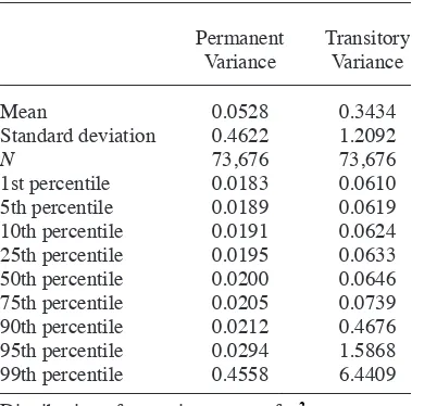
Table 4 presents the basic parameter estimates obtained from fi tting our model to the PSID earnings data described in Section IIIC. The left panel shows the distribution of risk in the population, 2
and 2
. Formally, we present the distribution of posterior means of permanent and transitory variance parameters. The right panel shows the mapping from shocks to earnings changes, , which we constrained to be constant over time and across individuals.
Note the extreme skew and fat tails (kurtosis) in the distribution of volatility param-eters, 2, shown in the left panel of Table 4. Although medians are modest, means far
Table 4
Standard deviation 0.4622 1.2092
N 73,676 73,676
1st percentile 0.0183 0.0610
5th percentile 0.0189 0.0619
10th percentile 0.0191 0.0624
25th percentile 0.0195 0.0633
50th percentile 0.0200 0.0646
75th percentile 0.0205 0.0739
90th percentile 0.0212 0.4676
95th percentile 0.0294 1.5868
99th percentile 0.4558 6.4409
Distribution of posterior means of 2
Notes: The left panel presents the posterior mean estimates of the volatility parameters, 2
. The distributions presented here consider all years and all individuals together. The right panel of this table present , the map-ping of shocks to earnings changes.
Jensen and Shore 823
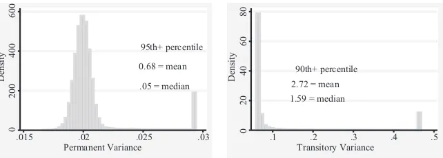
exceed medians. At the median, transitory shocks have a standard deviation of ap-proximately 25 percent annually; permanent shocks have a standard deviation of just under 14 percent annually. However, the highest volatility observations imply shocks with standard deviations well above 100 percent annually. Figure 2 plots these skewed and fat- tailed distributions by truncating the right tail.
As shown in the right panel of Table 4, permanent shocks enter in quickly (,k are close to one) while transitory shocks damp out quickly (,k fall to zero). Shocks were calibrated as a one standard deviation shock for an individual with volatility parame-ters at the estimated means (pulled from Table 4).
B. Evolution of the Volatility Distribution
Here, we show how the distribution of posterior means of variance parameters has evolved over time. This evolution is shown in Table 5 and also in Figure 3. Table 5 shows the year- by- year distribution of volatility parameters (t
2) posterior means.
This table mirrors Table 3, with volatility parameter (i2,t) posterior means replacing reduced form moments. The fi rst three columns show results for the permanent vari-ance parameter, 2; the
fi nal three columns show results for the transitory variance parameter, 2. The
fi rst and fourth columns present means of the permanent and transitory variance parameter posterior means, the second and fi fth columns present medians of parameter posterior means, and the third and sixth columns present 95th percentiles. The fi rst row shows whole- sample results. The second row shows the percent change in the mean, median, or 95th percentile over the sample.14 The
14. This is calculated as coeffi cient of a weighted OLS regression of the year- specifi c moments from below on a time trend, multiplied by the number of years (2009–1968), and divided by the whole- sample value in the previous row.
Distribution of Permanent and Transitory Variance
Notes: This fi gure presents the distribution of 2
and 2
The Journal of Human Resources
824
Table 5
Year- by- Year Volatility Parameters
Permanent Variance, 2 Transitory Variance,
2
Mean Median 95th Percent Mean Median 95th Percent
Average 0.0528 0.0200 0.0294 0.3434 0.0646 1.5868
Percent change 92 0.2 44 77 1 105
Slope 0.0012 0.0000 0.0003 0.0064 0.0000 0.0406
(t- statistic) (8.19) (4.08) (6.92) (5.89) (7.04) (4.75)
1970 0.0321 0.0200 0.0215 0.1961 0.0642 0.6794
1971 0.0351 0.0200 0.0223 0.2277 0.0644 0.7991
1972 0.0257 0.0200 0.0237 0.2382 0.0644 1.0918
1973 0.0447 0.0200 0.0237 0.2530 0.0645 1.0563
1974 0.0335 0.0200 0.0217 0.2127 0.0644 0.6554
1975 0.0450 0.0200 0.0237 0.2504 0.0645 1.0293
1976 0.0405 0.0200 0.0269 0.3297 0.0645 1.5216
1977 0.0388 0.0200 0.0253 0.3014 0.0644 1.3856
1978 0.0380 0.0200 0.0247 0.2494 0.0644 1.0520
1979 0.0539 0.0200 0.0262 0.2752 0.0645 1.2935
1980 0.0489 0.0200 0.0265 0.2607 0.0644 1.0971
1981 0.0450 0.0200 0.0258 0.2616 0.0645 1.0927
1982 0.0442 0.0200 0.0264 0.2982 0.0645 1.4414
1983 0.0505 0.0200 0.0309 0.3386 0.0646 1.8450
1984 0.0581 0.0200 0.0287 0.3074 0.0647 1.5723
1985 0.0389 0.0200 0.0260 0.3009 0.0646 1.3393
1986 0.0499 0.0200 0.0267 0.3249 0.0645 1.4454
Jensen and Shore
825
1988 0.0503 0.0200 0.0260 0.2802 0.0645 1.2503
1989 0.0442 0.0200 0.0276 0.2971 0.0644 1.5278
1990 0.0582 0.0200 0.0281 0.2868 0.0645 1.1882
1991 0.0444 0.0200 0.0285 0.3305 0.0646 1.5390
1992 0.0468 0.0200 0.0300 0.3168 0.0646 1.6275
1993 0.0613 0.0200 0.0380 0.5273 0.0649 3.0647
1994 0.0578 0.0200 0.0358 0.5257 0.0649 3.1216
1995 0.0519 0.0200 0.0345 0.4928 0.0648 2.5876
1996 0.0558 0.0200 0.0343 0.5072 0.0647 2.8367
1997 0.0542 0.0200 0.0335 0.4431 0.0647 2.3875
1999 0.0590 0.0200 0.0310 0.3645 0.0648 1.7913
2001 0.0600 0.0200 0.0286 0.3528 0.0648 1.5849
2003 0.0635 0.0200 0.0376 0.5501 0.0651 3.1466
2005 0.0978 0.0200 0.0324 0.3721 0.0647 1.9929
2007 0.0937 0.0200 0.0332 0.3884 0.0647 1.6072
2009 0.0764 0.0200 0.0298 0.4186 0.0654 1.8391
Notes: The construction of posterior means for 2 and
2
The Journal of Human Resources
90th and 95th Percentiles 90th and 95th Percentiles
≤75th Percentiles ≤75th Percentiles
90th Percentile Volatility 95th Percentile Volatility
.018
1st Percentile Polatility 5th Percentile Volatility 25th Percentile Volatility
90th Percentile Volatility 95th Percentile Volatility
1st Percentile Polatility 5th Percentile Volatility 25th Percentile Volatility 75th Percentile Volatility 10th Percentile Volatility
Median Volatility
Figure 3
Evolution of Percentiles of Volatility Distribution
Jensen and Shore 827
coeffi cient and t- statistic from this regression are shown just below. Year- by- year values are then shown.
Table 5 shows that the means of permanent and transitory parameters have increased substantially over the sample (by 92 and 77 percent, respectively) while the medians have not (0.2 and 1 percent increases, respectively). The qualitative results are robust to halving the bottom code and doubling the top code. This divergence can be explained by an increase in the magnitude of permanent and transitory variance parameters at the right tail among individuals with the highest parameters (the 95th percentile values increasing 44 percent and 105 percent, respectively). Colloquially, the kind of people whose earnings had always moved around a lot are moving around even more than they used to; the median person’s earnings do not move more than they used to.
This pattern can be seen graphically in Figure 3, which shows the year- by- year evolution of many quantiles of the distribution of permanent and transitory variance posterior means. In the bottom panels of Figure 3, we plot the 1st, 5th, 10th, 25th, 50th, and 75th percentile values of the posterior mean of the permanent (2, left) and transitory (2, right) variance parameters by year. These are very stable and show no clear upward trend. The size of this increase is extremely small economically. Looking at all but the “risky” tail of the distributions, the distributions look very stable.
In the middle and upper panels of Figure 3, we show the evolution of the “risky” tail of the distribution of posterior means. In this case, variance parameters increase strongly and signifi cantly. This increase in the right tail of the distribution explains the increase in the mean completely.
C. Heterogeneity or Fat Tails?
So far, we have shown that the increases in earnings volatility can be attributed solely to increases in the right tail of the volatility distribution. To obtain this result, our model assumes that the distribution of shocks is normal conditional on the volatil-ity parameters. When the unconditional distribution of shocks is fat tailed (has high kurtosis), this is automatically attributed to heterogeneity in volatility parameters. An alternative hypothesis is that there is little or no heterogeneity in volatility parameters but that shocks are conditionally fat tailed (Hirano 2002)15.
When looking at the cross- section of earnings changes, heterogeneity in volatil-ity parameters (with conditionally normal shocks) and conditionally fat- tailed shocks (without no heterogeneity in volatility parameters) are observationally equivalent; they both imply a fat- tailed unconditional distribution of earnings changes. By examining serial dependence, it is possible to reject the hypothesis that everyone has the same volatility parameter. If shocks are conditionally fat tailed but everyone has the same volatility parameters, then those with large past earnings changes should be no more likely than others to experience large subsequent earnings changes. If individuals dif-fer in their volatility parameters and those volatilities are persistent, then individuals with large past earnings changes will be more likely than others to have large subse-quent earnings changes.
The Journal of Human Resources 828
This possibility is investigated in Figure 1, comparing the sample variance of earn-ings changes for individuals with and without large past earnearn-ings changes. In each year, a cohort without large earnings changes is formed as the set of individuals whose measure of variance, either permanent variance or squared earnings change, was be-low median four years ago; a cohort with large earnings changes is formed as the set of individuals whose measure of variance was above the 95th percentile four years ago. This four- year period is chosen so that earnings shocks are far enough apart to be uncorrelated (Abowd and Card 1989).
Note that individuals with large past earnings changes tend to have larger subse-quent earnings changes. The tendency to have large earnings changes is persistent, which indicates that some individuals have ex ante more volatile earnings than others.
The divergence over time in volatility between past low- and high- volatility co-horts is clear in Figure 1. The magnitude of earnings changes has been increasing more for those with large past earnings changes (who are more likely to be inherently high- volatility) than for those without such large past earnings changes (who are not). This increase in volatility falls primarily on those who could be expected to have volatile earnings to begin with. This shows that the increase in volatility among the volatile we fi nd in the model cannot be attributed to increasingly fat- tailed shocks for everyone.
D. Whose Earnings Are Volatile?
In this paper, we have identifi ed increasing volatility for men in the United States since 1968 as being driven solely by the right (volatile) tail of the volatility distribution. Here, we examine the attributes of men with highly volatile earnings.
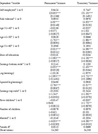
Table 6 presents the results from a probit regression to predict whether a person- year estimate of the (posterior mean) volatility parameter is above the 90th percentile for that year. Note from the fi rst row that self- employed individuals are much more likely to have highly volatile earnings. The second row shows that “risk- tolerant” individu-als are individu-also much more likely to have highly volatile earnings. Risk- tolerance is iden-tifi ed from answers to hypothetical questions about lotteries, designed to elicit the individual’s coeffi cient of relative risk- aversion; risk- tolerant individuals are defi ned as those with an estimated coeffi cient of relative risk- aversion below 1/0.3.
High earnings individuals (those with earnings above median four years before the observation in question) are less likely to have volatile earnings, with volatility fall-ing with earnfall-ings throughout the earnfall-ings distribution. Individuals with more years of education are also less likely to have volatile earnings. Older individuals are more likely to have volatile earnings, a result driven by the large number of high- volatility individuals between ages 50 and 60. Unsurprisingly, men who are married and/or who have children are less likely to have volatile earnings.
E. Whose Earnings Are Increasingly Volatile?
Jensen and Shore 829
Table 6
Determinants of High Volatility (Probit)
Dependent Variable Permanent Variance Transitory Variance
Self- employed? 1 or 0 0.6424 0.7447 (26.63)*** (31.15)***
[0.1266] [0.1491] Risk- tolerant? 1 or 0 0.0953 0.0970
(4.6)*** (4.63)*** [0.0140] [0.0138]
Age 31–40? 1 or 0 –0.0186 –0.0337
(–0.57) (–1.02)
[–0.0027] [–0.0047]
Age 41–50? 1 or 0 0.0620 0.0666
(1.78)** (1.90)** [0.0091] [0.0094]
Age 51–60? 1 or 0 0.1968 0.1932
(5.01)*** (4.89)*** [0.0311] [0.0295]
Years of education –0.0118 –0.0184
(–2.68)*** (–4.16)*** [–0.0017] [–0.0026] Earnings bottom code? 1 or 0 0.2141 0.1285
(4.03)*** (2.45)***
[0.0320] [0.0164]
Log(earnings) –1.0126 –1.9375
(–2.95)*** (–5.72)*** [–0.1461] [–0.2696] Squared log(earnings) 0.0468 0.0920
(2.76)*** (5.5)*** [0.0067] [0.0128] Earnings top code? 1 or 0 –0.2502 –0.3424
(–1.34)* (–1.88)** [–0.0301] [–0.0370] Have children? 1 or 0 –0.0147 –0.0557
(–046) (–1.73)**
[–0.0021] [–0.0079]
Number of children –0.0079 0.0070
(–0.62) (0.55)
[–0.0011] [0.0010]
Married? 1 or 0 –0.1848 –0.2034
(–6.03)*** (–6.59)*** [–0.0293] [–0.0315]
Pseudo- R2 0.0523 0.0699
Observations 34,363 34,363
The Journal of Human Resources 830
Table 7 predicts the posterior mean variance (volatility) estimates described earlier with a linear time trend. The “change” row shows the coeffi cient on calendar time; the “percent change” row shows the expected percent change over the sample implied by this coeffi cient. The top panel presents results for the permanent variance; the bottom panel presents results for the transitory variance. Each column presents results for a different subsample. By comparing the fi rst two columns, note that that volatility has increased dramatically more for self- employed people than for others. These indi-viduals have much higher average levels of volatility but their percentage change in volatility is still higher than for other individuals. Self- employed individuals account for a substantial proportion of the overall increase in earnings volatility. Similarly, the increase in permanent volatility (the variance of permanent shocks) is much greater for those who self- identify as risk- tolerant (those whose estimated coeffi cient of rela-tive risk aversion less than 1 / 0.3) than those who do not. Transitory volatility does not show major differences in trend for risk- tolerant and not risk- tolerant individuals.
Table 7 shows that the increase in volatility is apparent throughout the earnings distribution. While increases in the average variance of transitory shocks are similar (in proportional terms) for those with above- and below- median earnings, the variance of permanent shocks has increased more for those with above- median earnings than for those with below- median earnings. While below- median individuals are over-represented among those with the highest volatilities (Section IVE), low- earning in-dividuals are not driving the increase in volatility among those with the most volatile earnings.
Table 8 presents results by age and educational attainment. Note that while mag-nitudes vary, the increase in volatility at the right tail is present for those below and above 40 and across the education distribution.
V. Conclusion
Increases in the magnitude of earnings changes in the PSID can be at-tributed almost entirely to the “right tail” of the volatility distribution. Taking volatility as a proxy for risk, those who would have had risky earnings in the past now face even more risk. Everyone else has had no substantial change.
One way to frame the results in this paper is to assume that individuals face menus of risk- return options from which they choose the best career given their risk prefer-ences. Ceteris paribus, the most risk- tolerant people will select into the riskiest ca-reers. This selection provides a way of understanding why those with the most volatile earnings in the data also self- identify as risk- tolerant. In this setting, changes in the shape of this risk- return menu (or the distribution of risk- tolerance) will change the distribution of risk observed in the economy. We can then interpret the increase in earnings volatility among the most volatile as an increase in the returns to risk- taking at the top end. Without knowing more, the welfare implications of this fi nding are unclear.
Jensen and Shore
831
Table 7
Volatility Trends by Self- Employment, Earnings, and Risk- Tolerance
Self- Employment Earnings Risk Tolerance
Sample
Self- Employed
Not Self- Employed
> Median
Earnings ≤
Median Earnings
Risk- Tolerant
Not Risk- Tolerant
Permanent variance
Change per year 0.0046 0.0009 0.0006 0.0016 0.0021 0.0017
Percent change 1968 – 2009 266 72 82 83 160 160
(6.76)*** (5.52)*** (4.37)*** (5.53)*** (5.05)*** (7.26)***
N 6,069 45,177 25,443 25,803 11,131 18,964
Transitory variance
Change per year 0.0293 0.0064 0.0034 0.0108 0.0085 0.0073
Percent change 1968 – 2009 178 92 94 84 89 97
(11.09)*** (14.39)*** (9.94)*** (12.27)*** (6.54)*** (8.75)***
N 6,069 45,177 25,443 25,803 11,131 18,964
The Journal of Human Resources
832
Table 8
Volatility Trends by Age and Education
Age Education
Sample
Less than 40 Years Old
At Least 40 Years Old
More than
High School High School
Less than High School
Permanent variance
Mean change/year 0.0006 0.0013 0.0018 0.0003 0.0007
Percent change 1968–2009 70 75 134 24 55
(4.57)*** (4.69)*** (7.13)*** (1.14) (2.30)**
Median change/year 0.0000 0.0000 0.0000 0.0000 0.0000
Percent change 1968–2009 0 0 0 0 0
(–0.14) (0.64) (1.27) (–1.25) (1.8)*
95th percentile change/year 0.0003 0.0004 0.0004 0.0003 0.0003
Percent change 1968–2009 45 63 56 47 41
(9.67)*** (16.31)*** (10.32)*** (10.94)*** (5.90)***
Jensen and Shore
833
Transitory variance
Mean change/year 0.0059 0.0081 0.0083 0.0057 0.0066
Percent change 1968–2009 78 94 95 79 85
(9.55)*** (11.41)*** (10.87)*** (7.92)*** (6.92)***
Median change/year 0.0000 0.0000 0.0000 0.0000 0.0000
Percent change 1968–2009 1 1 1 2 2
(7.10)*** (13.76)*** (11.04)*** (09.89)*** (7.68)***
95th percentile change/year 0.0337 0.0565 0.0503 0.0455 0.0416
Percent change 1968–2009 98 89 132 144 107
(7.75)*** (11.48)*** (9.78)*** (9.37)*** (6.07)***
N 25,689 25,557 25,567 16,461 9,218
The Journal of Human Resources 834
in survey data refl ects increases in measured volatility for a minority of individu-als with volatile earnings; these individuindividu-als are more likely to be self- employed and risk- tolerant. This suggests that differences between survey and administrative data (and changes in those differences) in the way this group is measured may drive the diverging results. High- volatility individuals may think of year- to- year changes in their earnings differently than administrative records do; for example, the distinction between labor earnings and deferred compensation reinvested into a business may be particularly relevant for this group and changing over time. To the degree that this divergence has changed over time, it could explain the differences between results based on survey and administrative data.
References
Abowd, John, and David Card. 1989. “On the Covariance Structure of Earnings and Hours Changes.” Econometrica 57(2):411–45.
Altonji, Joseph G., Anthony Smith, and Ivan Vidangos. 2009. “Modeling Earnings Dynamics.” NBER Working Paper 14743.
Bania, Neil, and Laura Leete. 2007. “Income Volatility and Food Insuffi ciency in U.S. Low Income Households, 1992–2003.” Institute for Research on Poverty Discussion Paper Number 1325- 07.
Batchelder, Lily L. 2003. “Can Families Smooth Variable Earnings?” Harvard Journal on Legislation 40(2):395–452.
Blundell, Richard, Luigi Pistaferri, and Ian Preston. 2008. “Consumption Inequality and Partial Insurance.” American Economic Review 98(5):1887–921.
Bollinger, Christopher, Luis Gonzalez, and James P. Ziliak. 2009. “Welfare Reform and the Level and Composition of Income.” In Welfare Reform and its Long- Term Consequences for America’s Poor, ed. James P. Ziliak, 59–103. Cambridge, U.K.: Cambridge University Press.
Browning, Martin, Mette Ejrnæs, and Javier Alvarez. 2010. “Modelling Income Processes with Lots of Heterogeneity.” The Review of Economic Studies 77(4):1353–81.
Cameron, Stephen, and Joseph Tracy. 1998. “Earnings Variability in the United States: An Examination Using Matched- CPS Data.” Paper prepared for the 1998 Society of Labor Economics Conference.
Carroll, Christopher D., and Andrew A. Samwick. 1997. “The Nature of Precautionary Wealth.” Journal of Monetary Economics 40(1):41–71.
Comin, Diego, Erica L. Groshen, and Bess Rabin. 2009. “Turbulent Firms, Turbulent Wages?”
Journal of Monetary Economics 56:109–33.
Dahl, Molly, Thomas DeLeire, and Jonathan A. Schwabish. 2011. “Estimates of Year- to- Year Volatility in Earnings and in Household Incomes from Administrative, Survey, and Matched Data.” Journal of Human Resources 46(4):750–74.
Daly, Mary C., and Greg J. Duncan. 1997. “Earnings Mobility and Instability, 1969–1995.” Working Papers in Applied Economic Theory Number 97- 06. Federal Reserve Bank of San Francisco.
DeBacker, Jason, Bradley Heim, Vasia Panousi, Shanthi Ramnath, and Ivan Vidangos. 2012. “The Properties of Income Risk in Privately Held Businesses.” Board of Governors of the Federal Reserve System (U.S.), Finance and Economics Discussion Series: 2012- 69. ———. 2013. “Rising Inequality: Transitory or Persistent? New Evidence from a Panel of U.S.
Jensen and Shore 835
Dynan, Karen E., Douglas W. Elmendorf, and Daniel E. Sichel. 2007. “The Evolution of Earn-ings and Income Volatility.” FEDS Working Paper Number 2007- 61.
———. 2012. “The Evolution of Household Income Volatility.” The B.E. Journal of Economic Analysis and Policy 12(2).
Dynarski, Susan, and Jonathan Gruber. 1997. “Can Families Smooth Variable Earnings?”
Brookings Papers on Economic Activity 1:229–303.
Geman, S., and D. Geman. 1984. “Stochastic Relaxation, Gibbs Distributions, and the Bayesian Restoration of Images.” IEEE Transaction on Pattern Analysis and Machine Intelligence 6:721–41.
Geweke, John F., and Michael Keane. 2000. “An Empirical Analysis of Income Dynamics Among Men in the PSID: 1968–1989.” Journal of Econometrics 96:293–356.
Gorbachev, Olga. 2011. “Did Household Consumption Become More Volatile?” The American Economic Review 101(5):2248–70.
Gottschalk, Peter, and Robert Moffi tt. 1994. “The Growth of Earnings Instability in the U.S. Labor Market.” Brookings Papers on Economic Activity 2:217–54.
———. 2002. “Trends in the Transitory Variance of Earnings in the United States.” Economic Journal 112:C68–73.
———. “Trends in Earnings Volatility in the U.S.: 1970–2002.” Paper presented at the Meeting of the American Economic Association, Chicago, January 2007.
———. 2009. “The Rising Instability of U.S. Earnings. Journal of Economic Perspectives 23:3–24. Guvenen, Fatih, Serdar Ozkan, and Jae Song. 2012. “The Nature of Countercyclical Income
Risk.” NBER Working Paper 18035.
Hacker, Jacob. 2006. The Great Risk Shift: The Assault on American Jobs, Families, Health Care, and Retirement and How You Can Fight Back. Oxford: Oxford University Press. Haider, Steven J. “Earnings Instability and Earnings Inequality in the United States, 1967–
1991.” Journal of Labor Economics 19(4):799–836.
Hertz, Tom. 2006. “Understanding Mobility in America.” Center for American Progress Discussion Paper. Washington D.C. http://cdn.americanprogress.org/wp- content/uploads/kf/ hertz_mobility_analysis.pdf
Hirano, Keisuke. 2002. “Semiparametric Bayesian Inference in Autoregressive Panel Data Models.” Econometrica 70:781–99.
Hyslop, Dean R. 2001. “Rising U.S. Earnings Inequality and Family Labor Supply: The Cova-riance Structure of Intrafamily Earnings.” American Economic Review 91(4):755–77. Jensen, Shane T., and Stephen H. Shore. 2011. “Semi- Parametric Bayesian Modelling
of Income Volatility Heterogeneity.” Journal of the American Statistical Association
106(496):1280–90.
Keys, Benjamin J. 2008. “Trends in Income and Consumption Volatility.” In Income Volatil-ity and Food Assistance in the United States, ed. Dean Jolliffe and James P. Ziliak, 11–34. Kalamazoo: W.E. Upjohn Institute.
Little, Roderick J.A., and Donald B. Rubin. 2002. Statistical Analysis with Missing Data, 2nd Edition. New York: Wiley Interscience.
Meghir, Costas, and Luigi Pistaferri. 2004. “Income Variance Dynamics and Heterogeneity.”
Econometrica 72(1):1–32.
Moffi tt, Robert A., and Peter Gottschalk. 2011. “Trends in the Covariance Structure of Earn-ings in the U.S.” Journal of Economic Inequality 9:439–59.
Rao, J.N.K., and J. Shao. 1992. “Jackknife Variance Estimation with Survey Data Under Hot Deck Imputation.” Biometrika 79(4):811–22.
Reilly, Marie. 1993. “Data Analysis Using Hot Deck Multiple Imputation.” Journal of the Royal Statistical Society. Series D (The Statistician) 42(3):307–13.
The Journal of Human Resources 836
———. 2010. “The Great Moderation in Micro Labor Earnings.” Journal of Monetary Econom-ics 57:391–403.
Shin, Dongyun, and Gary Solon. 2011. “Trends in Men’s Earnings Volatility: What Does the Panel Study of Income Dynamics Show?” Journal of Public Economics 95(7):973–82. Shore, Stephen H. 2010. “For Better, for Worse: Intrahousehold Risk- Sharing over the
Busi-ness Cycle.” The Review of Economics and Statistics 92(3):536–48.
Storesletten, Kjetil, Chris I. Telmer, and Amir Yaron. 2004. “Cyclical Dynamics in Idiosyn-cratic Labor Market Risk.” Journal of Political Economy 112(3):695–717.
Teh, Y., M. Jordan, M. Beal, and D. Blei. 2007 “Hierarchical Dirichlet Processes.” Journal of the American Statistical Association 101(476):1566–81.
Winship, Scott. 2007. “Income Volatility, the Great Risk Shift, and the Democratic Agenda.” Technical report, Unpublished.