Finite volume numerical solution to a blood flow problem in human artery.

(1)

(2)

This content has been downloaded from IOPscience. Please scroll down to see the full text.

Download details:

IP Address: 202.94.83.84

This content was downloaded on 11/02/2017 at 06:17

Please note that terms and conditions apply.

Finite volume numerical solution to a blood flow problem in human artery

View the table of contents for this issue, or go to the journal homepage for more

(3)

Finite volume numerical solution to a blood flow problem in

human artery

Inge Wijayanti Budiawan and Sudi Mungkasi

Department of Mathematics, Faculty of Science and Technology,

Sanata Dharma University, Mrican, Tromol Pos 29, Yogyakarta 55002, Indonesia

E-mail: theresia.inge0303@gmail.com, sudi@usd.ac.id

Abstract. In this paper, we solve a one dimensional blood flow model in human artery. This model is of a non-linear hyperbolic partial differential equation system which can generate either continuous or discontinuous solution. We use the Lax–Friedrichs finite volume method to solve this model. Particularly, we investigate how a pulse propagates in human artery. For this simulation, we give a single sine wave with a small time period as an impluse input on the left boundary. The finite volume method is successful in simulating how the pulse propagates in the artery. It detects the positions of the pulse for the whole time period.

1. Introduction

Blood is one of body components which has important functions. One of blood functions is to distribute the nutritions to all human body tissues. In some cases, blood flow may be hindered because of some problems, such as plugging and artery cavity stiffening [1-2]. It is a dangerous condition that must be overcome. In this case, medical treatment can affect the blood flow pattern. Blood flow in human artery can be represented in a mathematical model. We can investigate blood flow patterns from the solution of its model [3-5]. Numerical methods are considered, as they are powerful [6-8] to solve mathematical models.

In this paper, our focusses are to find and simulate numerical solution of the one dimensional blood flow model in human artery. There are a number of methods which can be used to solve this model, but we use the Lax–Friedrichs finite volume method [9-12] because of its simplicity. Moreover, finite volume methods can be used to find either continuous or discontinuous solution [13-14].

The paper is organised as follows. Section 2 gives the problem that we want to solve. Research method is presented in Section 3. Numerical results are provided in Section 4. Conclusion is drawn in Section 5.

2. Problem formulation

In this section, we describe the problem of blood flow in human artery, which we want to solve. We consider a straight cylindrical tube with circular cross section and z coordinate is the axis of cylinder (see Figure 1). The one dimensional blood flow model for human artery [2] is

+ = 0 , (1)

+ ∝ + + = 0 , (2)

ICSAS IOP Publishing

IOP Conf. Series: Journal of Physics: Conf. Series 795(2017) 012042 doi:10.1088/1742-6596/795/1/012042

Content from this work may be used under the terms of theCreative Commons Attribution 3.0 licence. Any further distribution of this work must maintain attribution to the author(s) and the title of the work, journal citation and DOI.

(4)

for ∈ 0, and > 0, where , , and are the cross section area of artery, the blood discharge, and the blood pressure, respectively. In addition, ∝ is the velocity function in every cross section artery which is assumed as a constant (in this paper we set its value equals to one), is the density of blood, is the coefficient which relates to the blood viscosity, is the space variable, and is the time variable.

Figure 1. Ilustration of human artery.

In this model, there are three dependent variables ( , , dan ) and two equations. In order to have two equations with two unknowns, we define a relation that links the blood pressure with the cross section area of artery

= + − ! . (3)

Here _#$% is the external pressure and is the artery cross section area at initial time = 0. In this paper, is assumed to be zero and is constant. Furthermore, is a parameter relating to the artery wall elastic properties:

=4 'ℎ₃ ) , (4)

where ) is the elastic Young’s modulus.

3. Numerical method

In this section, we explain the finite volume method for solving blood flow model (1)-(2). We use the flux formulation of Lax–Friedrichs [9].

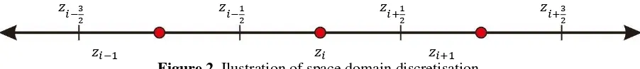
To find numerical solutions of this blood flow model, let us consider the space domain discretisation (as shown in Figure 2) where ∆ = _,-./ − _,0./ or ∆ = _,− _,0., and the time domain discretisation 1= 2 ∆ for integers 2.

,03₄ ,05₄ ,-5₄ ,-3₄

,0. , ,-.

Figure 2. Ilustration of space domain discretisation.

From equation (3), we obtain

= 6 − !7

=8₈ 54+ 2 054 −8 8

5 4_.

If we multiply both sides of the previous equation with / , we get

(5)

=8₈

Based on equation (7), equation (2) can be rewritten as

+ _{+ 3} 34 = − + 8

8 < −23 =. (8)

From the above derivation, blood flow model (1)-(2) are balance laws in the form of

>?%+ @? >? A = B? >? (9)

where the conserved quantities, flux functions, and source terms are

>? = C D, @? >? = EF4 The fully discrete finite volume method [9] to get the numerical solution to balance laws (9) is

OP,1-.= OP,1−_{∆ <W}∆ P_,-5 4 1 _{− WP}

,015₄= + ∆ R?,1 , (10)

with the definition of the Lax–Friedrichs flux

WP_,-5

From the finite volume scheme (10)-(12), we get the numerical scheme for blood flow model (1)-(2) as follows. The numerical scheme for equation (1) is

, 1-.₌

, 1₋∆

∆ <W,-15₄− W,015₄= , (13)

with the definition of Lax–Friedrichs fluxes W_,-5

In addition, the numerical scheme for equation (2) is

(6)

with the definition of Lax–Friedr We are now ready to present our r

4. Numerical simulation nearest point from the heart and of coefficients that we use in all s

Table 1. in the form of a single sine wave w

= 0 our results of numerical simulations of the blood flow

how a pulse propagates in human artery. Numerica n as follow.

A layout of human artery for numerical simulation.

e monitoring points (P, M, and D) for the pressur al, medium, and distal points, respectively. Conside nd point a is the farthest point from the heart. Tabl

ll simulations.

1. Coefficients value for numerical simulation.

oefficient Value ation is taken as follows. At the left boundary, we g

(7)

For the left boundary value of and , let us consider the characteristic variables of model (1)-(2) which has been explained in [2]: i_. and i are given by

i = − 2j2 5k , (20)

i.= i + 4j2 [ + , (21)

= < = i.− i₄_m l , (22)

= i.+ i₂ . (23)

We set i as a constant and equals to its initial value. And the last, for each right boundary value of , and equals to the corresponding value of the nearest neighbour in the domain.

4.3. Numerical results

In this subsection, we summarise our numerical results.

Figure 4. Graphics of the artery cross section area with respect to time.

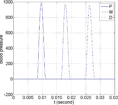
Figure 5. Graphics of the blood presure with respect to time.

Figure 6. Graphics of the artery cross section area with respect to space.

Figure 7. Graphics of the blood pressure with respect to space.

(8)

For this numerical simulation, where the elastic Young’s modulus is constant, the blood pressure is directly propotional with the artery cross section area (see Figure 4 and Figure 6). Furthermore, the blood pressure amplitude decreases with respect to time and space (see Figure 5 and Figure 7). We infer that the decrease is influenced by the dissipation of the numerical method. We note that as the cell width is taken smaller, the amplitude can be maintained almost the same as the original one, as long as the solution is continuous.

5. Conclusion

Based on the numerical results, the form of pulse does not change but the amplitude decreases with respect to time and space due to numerical dissipation. The dissipation can be small if the numerical cell width is small. This research is limited to problems solved using the first order Lax–Friedrichs finite volume method. Future work could extend the method to higher order ones.

Acknowledgment

This work was financially supported by Sanata Dharma University. The financial support is gratefully acknowledged by both authors.

References

[1] Acosta A, Puelz C, Penny D J and Rusin C G 2015 Numerical method of characteristics for one-dimensional blood

flow Journal of Computational Physics 294 96

[2] Formaggia L, Nobile F and Quarteroni A 2002 A one dimensional model for blood flow: application to vascular

prosthesis, in Babuška I, et al. (eds.), Mathematical Modeling and Numerical Simulation in Continuum

Mechanics pp. 137-153 (Springer, Berlin)

[3] Montecinos G I, Müller L O and Toro E F 2014 Hyperbolic reformulation of a 1D viscoelastic blood flow model and

ADER finite volume schemes Journal of Computational Physics 266 101

[4] Müller L O and Toro E F 2013 Well-balanced high-order solver for blood flow in networks of vessels with variable

properties International Journal for Numerical Methods in Biomedical Engineering 29 1388

[5] Watanabe S M, Blanco P J, and Feijóo R A 2013 Mathematical model of blood flow in an anatomically detailed

arterial network of the arm ESAIM: M2AN 47 961

[6] Malik O U, Hilderman R J, Hamilton H J and Dosselmann R 2016 Retail price time series imputation International

Journal of Business Intelligence and Data Mining11 49

[7] Lu Z, Yan J and Wang X 2015 Using grouping strategy and pattern discovery for delta extraction in a limited

collaborative environment International Journal of Business Intelligence and Data Mining10 378

[8] Nesticò A and Pipolo O 2015 A protocol for sustainable building interventions: financial analysis and environmental

effects International Journal of Business Intelligence and Data Mining10 199

[9] LeVeque R J 2002 Finite Volume Methods for Hyperbolic Problems (Cambridge University Press, Cambridge)

[10] Mungkasi S 2016 An adaptive mesh finite volume method for the Euler equations of gas dynamics AIP Conference

Proceedings1737 040002

[11] Mungkasi S and Ningrum G I J 2016 Numerical solution to the linear acoustics equations AIP Conference

Proceedings1746 020056

[12] Mungkasi S and Sari I P 2016 Numerical solution to the shallow water equations using explicit and implicit schemes

AIP Conference Proceedings1746 020064

[13] Mungkasi S 2016 Adaptive finite volume method for the shallow water equations on triangular grids Advances in

Mathematical Physics2016 7528625

[14] Supriyadi B and Mungkasi S 2016 Finite volume numerical solvers for non-linear elasticity in heterogeneous media

International Journal for Multiscale Computational Engineering14 479