M O D E R N
P H Y S I C S
Third edition
K e n n e t h S. K r a n e
D E P A R T M E N T O F P H Y S I C S
O R E G O N S T A T E U N I V E R S I T Y
Chapter
4
THE WAVELIKE PROPERTIES OF
PARTICLES
In classical physics, the laws describing the behavior of waves and parti-cles are fundamentally different. Projectiles obey particle-type laws, such as Newtonian mechanics. Waves undergo interference and diffraction, which cannot be explained by the Newtonian mechanics associated with particles. The energy carried by a particle is confined to a small region of space; a wave, on the other hand, distributes its energy throughout space in its wavefronts. In describing the behavior of a particle we often want to specify its location, but this is not so easy to do for a wave. How would you describe the exact location of a sound wave or a water wave?
In contrast to this clear distinction found in classical physics, quantum physics requires that particles sometimes obey the rules that we have previously established for waves, and we shall use some of the language associated with waves to describe particles. The system of mechanics associated with quantum systems is sometimes called “wave mechanics” because it deals with the wavelike behavior of particles. In this chapter we discuss the experimental evidence in support of this wavelike behavior for particles such as electrons.
As you study this chapter, notice the frequent references to such terms as the
probability of the outcome of a measurement, theaverageof many repetitions of a measurement, and the statistical behavior of a system. These terms are fundamental to quantum mechanics, and you cannot begin to understand quantum behavior until you feel comfortable with discarding such classical notions as fixed trajectories and certainty of outcome, while substituting the quantum mechanical notions of probability and statistically distributed outcomes.
4.1 DE BROGLIE’S HYPOTHESIS
Progress in physics often can be characterized by long periods of experimental and theoretical drudgery punctuated occasionally by flashes of insight that cause profound changes in the way we view the universe. Frequently the more profound the insight and the bolder the initial step, the simpler it seems in historical perspective, and the more likely we are to sit back and wonder, “Why didn’t I think of that?” Einstein’s special theory of relativity is one example of such insight; the hypothesis of the Frenchman Louis de Broglie is another.∗
Louis de Broglie (1892–1987, France). A member of an aristocratic family, his work contributed substan-tially to the early development of the quantum theory.
In the previous chapter we discussed the double-slit experiment (which can be understood only if light behaves as a wave) and the photoelectric and Compton effects (which can be understood only if light behaves as a particle). Is this dual particle-wave nature a property only of light or of material objects as well? In a bold and daring hypothesis in his 1924 doctoral dissertation, de Broglie chose the latter alternative. Examining Eq. 3.20,E = hf,and Eq. 3.22,p=h/λ, we find some difficulty in applying the first equation in the case of particles, for we cannot be sure whetherEshould be the kinetic energy, total energy, or total relativistic energy (all, of course, are identical for light). No such difficulties arise from the second relationship. De Broglie suggested, lacking any experimental evidence in
∗De Broglie’s name should be pronounced “deh-BROY” or “deh-BROY-eh,” but it is often said as
4.1 | De Broglie’s Hypothesis 103
support of his hypothesis, that associated with any material particle moving with momentumpthere is a wave of wavelengthλ, related topaccording to
λ= h
p (4.1)
wherehis Planck’s constant. The wavelengthλof a particle computed according to Eq. 4.1 is called itsde Broglie wavelength.
Example 4.1
Compute the de Broglie wavelength of the following: (a) A 1000-kg automobile traveling at 100 m/s (about 200 mi/h). (b) A 10-g bullet traveling at 500 m/s. (c) A smoke particle of mass 10−9 g moving at 1 cm/s. (d) An electron with
a kinetic energy of 1 eV. (e) An electron with a kinetic energy of 100 MeV.
Solution
(a) Using the classical relation between velocity and momentum,
Because the kinetic energy (1 eV) is much less than the rest energy, we can use nonrelativistic kinematics.
p=√2mK
We can also find this solution in the following way, using
p=√2mKandhc=1240 eV·nm.
This method may seem artificial at first, but with prac-tice it becomes quite useful, especially because energies are usually given in electron-volts in atomic and nuclear physics.
(e) In this case, the kinetic energy is much greater than the rest energy, and so we are in the extreme relativistic realm, whereK∼=E∼=pc, as in Eq. 2.40. The wavelength is observed in the laboratory. Only in the last two cases, in which the wavelength is of the same order as atomic or nuclear sizes, do we have any chance of observing the wavelength. Because of the smallness of h, only for particles of atomic or nuclear size will the wave behavior be observable.
wave measure? We’ll discuss the answer to this question later in this chapter. For now, we assume that, associated with the particle as it moves, there is a de Broglie wave of wavelengthλ, which shows itselfwhen a wave-type experiment (such as diffraction) is performed on it.The outcome of the wave-type experiment depends on this wavelength. The de Broglie wavelength, which characterizes the wave-type behavior of particles, is central to the quantum theory.
The second question then occurs: Why was this wavelength not directly observed before de Broglie’s time? As parts (a), (b), and (c) of Example 4.1 showed, for ordinary objects the de Broglie wavelength is very small. Suppose we tried to demonstrate the wave nature of these objects through a double-slit type of experiment. Recall from Eq. 3.16 that the spacing between adjacent fringes in a double-slit experiment isy=λD/d. Putting in reasonable values for the slit separation d and slit-to-screen distance D, you will find that there is no achievable experimental configuration that can produce an observable separation of the fringes (see Problem 9). There is no experiment that can be done to reveal the wave nature of macroscopic (laboratory-sized) objects.Experimental verification of de Broglie’s hypothesis comes only from experiments with objects on the atomic scale, which are discussed in the next section.
4.2 EXPERIMENTAL EVIDENCE FOR
DE BROGLIE WAVES
The indications of wave behavior come mostly from interference and diffraction experiments. Double-slit interference, which was reviewed in Section 3.1, is perhaps the most familiar type of interference experiment, but the experimental difficulties of constructing double slits to do interference experiments with beams of atomic or subatomic particles were not solved until long after the time of de Broglie’s hypothesis. We discuss these experiments later in this section. First we’ll discuss diffraction experiments with electrons.
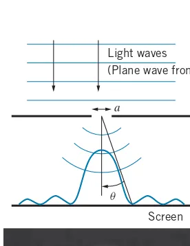
Light waves (Plane wave fronts)
a
Screen q
FIGURE 4.1 Light waves
(repre-sented as plane wave fronts) are inci-dent on a narrow slit of width a. Diffraction causes the waves to spread after passing through the slit, and the intensity varies along the screen. The photograph shows the resulting inten-sity pattern.
Particle Diffraction Experiments
Diffraction of light waves is discussed in most introductory physics texts and is illustrated in Figure 4.1 for light diffracted by a single slit. For light of wavelength
λincident on a slit of widtha, the diffraction minima are located at angles given by
asinθ=nλ n=1, 2, 3,. . . (4.2) on either side of the central maximum. Note that most of the light intensity falls in the central maximum.
The experiments that first verified de Broglie’s hypothesis involveelectron diffraction,not through an artificially constructed single slit (as for the diffraction pattern in Figure 4.1) but instead through the atoms of a crystal. The outcomes of these experiments resemble those of the similar X-ray diffraction experiments illustrated in Section 3.1.
In an electron diffraction experiment, a beam of electrons is accelerated from rest through a potential differenceV, acquiring a nonrelativistic kinetic energy
4.2 | Experimental Evidence for De Broglie Waves 105
crystal, and the scattered beam is photographed (Figure 4.2). The similarity between electron diffraction patterns (Figure 4.2) and X-ray diffraction patterns (Figure 3.7) strongly suggests that the electrons are behaving as waves.
Crystal Electron beam
Screen
FIGURE 4.2 (Top) Electron
diffrac-tion apparatus. (Bottom) Electron diffraction pattern. Each bright dot is a region of constructive interference, as in the X-ray diffraction patterns of Figure 3.7. The target is a crystal of Ti2Nb10O29.
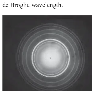
The “rings” produced in X-ray diffraction of polycrystalline materials (Figure 3.8b) are also produced in electron diffraction, as shown in Figure 4.3, again providing strong evidence for the similarity in the wave behavior of electrons and X rays. Experiments of the type illustrated in Figure 4.3 were first done in 1927 by G. P. Thomson, who shared the 1937 Nobel Prize for this work. (Thomson’s father, J. J. Thomson, received the 1906 Nobel Prize for his discovery of the electron and measurement of its charge-to-mass ratio. Thus it can be said that Thomson, the father, discovered the particle nature of the electron, while Thomson, the son, discovered its wave nature.)
An electron diffraction experiment gave the first experimental confirmation of the wave nature of electrons (and the quantitative confirmation of the de Broglie relationship λ=h/p) soon after de Broglie’s original hypothesis. In 1926, at the Bell Telephone Laboratories, Clinton Davisson and Lester Germer were investigating the reflection of electron beams from the surface of nickel crystals. A schematic view of their apparatus is shown in Figure 4.4. A beam of electrons from a heated filament is accelerated through a potential differenceV. After passing through a small aperture, the beam strikes a single crystal of nickel. Electrons are scattered in all directions by the atoms of the crystal, some of them striking a detector, which can be moved to any angleφrelative to the incident beam and which measures the intensity of the electron beam scattered at that angle. Figure 4.5 shows the results of one of the experiments of Davisson and Germer. When the accelerating voltage is set at 54 V, there is an intense reflection of the beam at the angleφ=50◦. Let’s see how these results give confirmation of the de Broglie wavelength.
FIGURE 4.3 Electron diffraction of
polycrystalline beryllium. Note the sim-ilarity between this pattern and the pattern for X-ray diffraction of a poly-crystalline material (Figure 3.8b).
Electron beam
Crystal
Detector
f
+V
F
FIGURE 4.4 Apparatus used by
Davisson and Germer to study electron diffraction. Electrons leave the filamentFand are accel-erated by the voltageV. The beam strikes a crystal and the scattered beam is detected at an angle φ
relative to the incident beam. The detector can be moved in the range 0 to 90◦.
f=50°
FIGURE 4.5 Results of Davisson
and Germer. Each point on the plot represents the relative intensity when the detector in Figure 4.4 is located at the corresponding angle
φmeasured from the vertical axis. Constructive interference causes the intensity of the reflected beam to reach a maximum atφ=50◦for
Incident
FIGURE 4.6 The crystal surface acts
like a diffraction grating with spac-ingd.
FIGURE 4.7 Diffraction of neutrons
by a sodium chloride crystal.
101
FIGURE 4.8 Diffraction of 1-GeV
protons by oxygen nuclei. The pat-tern of maxima and minima is similar to that of single-slit diffraction of light waves. [Source: H. Palevsky et al.,Physical Review Letters18, 1200 (1967).]
Each of the atoms of the crystal can act as a scatterer, so the scatteredelectron waves can interfere, and we have a crystal diffraction grating for the electrons. Figure 4.6 shows a simplified representation of the nickel crystal used in the Davisson-Germer experiment. Because the electrons were of low energy, they did not penetrate very far into the crystal, and it is sufficient to consider the diffraction to take place in the plane of atoms on the surface. The situation is entirely similar to using a reflection-type diffraction grating for light; the spacingdbetween the rows of atoms on the crystal is analogous to the spacing between the slits in the optical grating. The maxima for a diffraction grating occur at anglesφsuch that the path difference between adjacent raysdsinφis equal to a whole number of wavelengths:
dsinφ=nλ n=1, 2, 3,. . . (4.3)
wherenis the order number of the maximum.
From independent data, it is known that the spacing between the rows of atoms in a nickel crystal is d=0.215 nm. The peak at φ=50◦ must be a first-order peak (n=1), because no peaks were observed at smaller angles. If this is indeed an interference maximum, the corresponding wavelength is, from Eq. 4.3,
λ=dsinφ=(0.215 nm)(sin 50◦)=0.165 nm
We can compare this value with that expected on the basis of the de Broglie theory. An electron accelerated through a potential difference of 54 V has a kinetic energy of 54 eV and therefore a momentum of
p=√2mK= 1
This is in excellent agreement with the value found from the diffraction maxi-mum, and provides strong evidence in favor of the de Broglie theory. For this experimental work, Davisson shared the 1937 Nobel Prize with G. P. Thomson.
The wave nature of particles is not exclusive to electrons;anyparticle with momentumphas de Broglie wavelengthh/p. Neutrons are produced in nuclear reactors with kinetic energies corresponding to wavelengths of roughly 0.1 nm; these also should be suitable for diffraction by crystals. Figure 4.7 shows that diffraction of neutrons by a salt crystal produces the same characteristic patterns as the diffraction of electrons or X rays. Clifford Shull shared the 1994 Nobel Prize for the development of the neutron diffraction technique.
4.2 | Experimental Evidence for De Broglie Waves 107
Example 4.2
Protons of kinetic energy 1.00 GeV were diffracted by oxygen nuclei, which have a radius of 3.0 fm, to produce the data shown in Figure 4.8. Calculate the expected angles where the first three diffraction minima should appear.
Solution
The total relativistic energy of the protons is E= K+mc2
The corresponding de Broglie wavelength is
λ=h
We can represent the oxygen nuclei as circular disks, for which the diffraction formula is a bit different from Eq. 4.2:
asinθ=1.22nλ, whereais the diameter of the diffracting object. Based on this formula, the first diffraction minimum (n=1) should appear at the angle minimum should appear at the angle where sin
θ=2×0.148=0.296(θ=17.2◦), and then=3 minimum where sinθ=3×0.148=0.444(θ=26.4◦).
From the data in Figure 4.8, we see the first diffraction minimum at an angle of about 10◦, the second at about 18◦, and the third at about 27◦, all in very good agreement with the expected values. The data don’t exactly follow the formula for diffraction by a disk, because nuclei don’t behave quite like disks. In particular, they have diffuse rather than sharp edges, which prevents the intensity at the diffraction minima from falling to zero and also alters slightly the locations of the minima.
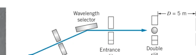
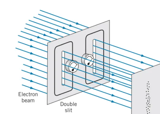
Double-Slit Experiments with Particles
The definitive evidence for the wave nature of light was deduced from the double-slit experiment performed by Thomas Young in 1801 (discussed in Section 3.1). In principle, it should be possible to do double-slit experiments withparticlesand thereby directly observe their wavelike behavior. However, the technological difficulties of producing double slits for particles are formidable, and such experiments did not become possible until long after the time of de Broglie. The first double-slit experiment with electrons was done in 1961. A diagram of the apparatus is shown in Figure 4.9. The electrons from a hot filament were accelerated through 50 kV (corresponding toλ=5.4 pm) and then passed through a double slit of separation 2.0μm and width 0.5μm. A photograph of the resulting intensity pattern is shown in Figure 4.10. The similarity with the double-slit pattern for light (Figure 3.2) is striking.
Electrons
for electrons. Electrons from the fila-mentFare accelerated through 50 kV and pass through the double slit. They produce a visible pattern when they strike a fluorescent screen (like a TV screen), and the resulting pattern is photographed. A photograph is shown in Figure 4.10. [See C. Jonsson, Amer-ican Journal of Physics42, 4 (1974).]
D= 5 m
Entrance slit Neutron beam
Wavelength selector
Double slit
Scanning slit
Detector
FIGURE 4.11 Double-slit apparatus for neutrons. Thermal neutrons from a reactor
are incident on a crystal; scattering through a particular angle selects the energy of the neutrons. After passing through the double slit, the neutrons are counted by the scanning slit assembly, which moves laterally.
FIGURE 4.10 Double-slit
interfer-ence pattern for electrons.
another slit across the beam and measuring the intensity of neutrons passing through this “scanning slit.” Figure 4.12 shows the resulting pattern of intensity maxima and minima, which leaves no doubt that interference is occurring and that the neutrons have a corresponding wave nature. The wavelength can be deduced from the slit separation using Eq. 3.16 to obtain the spacing between adjacent maxima,y=yn+1−yn. Estimating the spacingyfrom Figure 4.12 to be about 75μm, we obtain
λ= dy
D =
(126μm)(75μm)
5 m =1.89 nm
This result agrees very well with the de Broglie wavelength of 1.85 nm selected for the neutron beam.
Scanning slit position
100 mm
Intensity
FIGURE 4.12 Intensity pattern
ob-served for double-slit interference with neutrons. The spacing between the maxima is about 75μm. [Source:
R. Gahler and A. Zeilinger,American Journal of Physics59, 316 (1991).]
It is also possible to do a similar experiment with atoms. In this case, a source of helium atoms formed a beam (of velocity corresponding to a kinetic energy of 0.020 eV) that passed through a double slit of separation 8μm and width 1μm. Again a scanning slit was used to measure the intensity of the beam passing through the double slit. Figure 4.13 shows the resulting intensity pattern. Although the results are not as dramatic as those for electrons and neutrons, there is clear evidence of interference maxima and minima, and the separation of the maxima gives a wavelength that is consistent with the de Broglie wavelength (see Problem 8).
10 mm
Scanning slit position
Intensity
FIGURE 4.13 Intensity pattern
ob-served for double-slit interference with helium atoms. [Source:O. Car-nal and J. Mlynek, Physical Review Letters66, 2689 (1991).]
Diffraction can be observed with even larger objects. Figure 4.14 shows the pattern produced by fullerene molecules (C60) in passing through a diffraction
grating with a spacing of d=100 nm. The diffraction pattern was observed at a distance of 1.2 m from the grating. Estimating the separation of the maxima in Figure 4.14 as 50μm, we get the angular separation of the maxima to be
θ≈tanθ=(50μm)/(1.2 m)=4.2×10⁻⁵rad, and thusλ
=dsinθ=4.2 pm. For C60molecules with a speed of 117 m/s used in this experiment, the expected
de Broglie wavelength is 4.7 pm, in good agreement with our estimate from the diffraction pattern.
In this chapter we have discussed several interference and diffraction experiments using different particles—electrons, protons, neutrons, atoms, and molecules. These experiments are not restricted to any particular type of particle or to any particular type of observation. They are examples of ageneral
4.2 | Experimental Evidence for De Broglie Waves 109
–150 –100
Intensity
–50 0
Detector position in mm
50 100 150
FIGURE 4.14Diffraction grating
pat-tern produced by C60 molecules. [Source: O. Nairz, M. Arndt, and A. Zeilinger, American Journal of Physics71, 319 (2003).]
FIGURE 4.15 The atomic structure
of solid benzene as deduced from neutron diffraction. The circles indi-cate contours of constant density. The black circles show the locations of the six carbon atoms that form the familiar benzene ring. The blue circles show the locations of the hydrogen atoms.
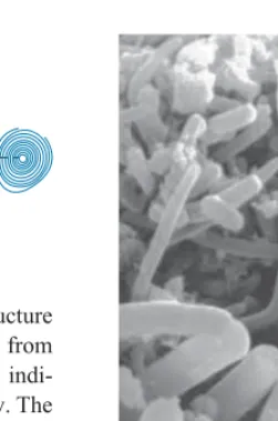
gives detailed information on the structure of solid crystals and of complex molecules (Figure 4.15). The electron microscope uses electron waves to illumi-nate and form an image of objects; because the wavelength can be made thousands of times smaller than that of visible light, it is possible to resolve and observe small details that are not observable with visible light (Figure 4.16).
FIGURE 4.16 Electron microscope
image of bacteria on the surface of a human tongue. The magnification here is about a factor of 5000.
Through Which Slit Does the Particle Pass?
When we do a double-slit experiment with particles such as electrons, it is tempting to try to determine through which slit the particle passes. For example, we could surround each slit with an electromagnetic loop that causes a meter to deflect whenever a charged particle or perhaps a particle with a magnetic moment passes through the loop (Figure 4.17). If we fired the particles through the slits at a slow enough rate, we could track each particle as it passed through one slit or the other and then appeared on the screen.
If we performed this imaginary experiment, the result would no longer be an interference pattern on the screen. Instead, we would observe a pattern similar to that shown in Figure 4.17, with “hits” in front of each slit, but no interference fringes. No matter what sort of device we use to determine through which slit the particle passes, the interference pattern will be destroyed. The classicalparticle
must pass through one slit or the other; only a wave can reveal interference, which depends on parts of the wavefront passing through both slits and then recombining.
When we ask through which slit the particle passed, we are investigating only theparticleaspects of its behavior, and we cannot observe its wave nature (the interference pattern). Conversely, when we study the wave nature, we cannot simultaneously observe the particle nature. The electron will behave as a particle
Electron beam
Double slit
Screen
FIGURE 4.17 Apparatus to record passage of electrons through slits.
Each slit is surrounded by a loop with a meter that signals the passage of an electron through the slit. No interference fringes are seen on the screen.
This is the basis for theprinciple of complementarity,which asserts that the complete description of a photon or a particle such as an electron cannot be made in terms of only particle properties or only wave properties, but that both aspects of its behavior must be considered. Moreover, the particle and wave natures cannot be observed simultaneously, and the type of behavior that we observe depends on the kind of experiment we are doing: a particle-type experiment shows only particle like behavior, and a wave-type experiment shows only wavelike behavior.
(a)
(b)
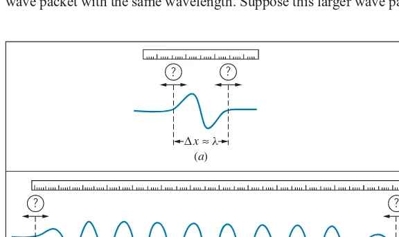
FIGURE 4.18 (a) A pure sine wave, which extends from −∞ to +∞. (b) A narrow wave pulse.
4.3 UNCERTAINTY RELATIONSHIPS FOR CLASSICAL
WAVES
4.3 | Uncertainty Relationships for Classical Waves 111
This competition between knowledge of location and knowledge of wavelength is not restricted to de Broglie waves—classical waves show the same effect. All real waves can be represented aswave packets—disturbances that are localized to a finite region of space. We will discuss more about constructing wave packets in Section 4.5. In this section we will examine this competition between specifying the location and the wavelength of classical waves more closely.
Figure 4.19ashows a very small wave packet. The disturbance is well localized to a small region of space of lengthx. (Imagine listening to a very short burst of sound, of such brief duration that it is hard for you to recognize the pitch or frequency of the wave.) Let’s try to measure the wavelength of this wave packet. Placing a measuring stick along the wave, we have some difficulty defining exactly where the wave starts and where it ends. Our measurement of the wavelength is therefore subject to a smalluncertaintyλ. Let’s represent this uncertainty as a fractionεof the wavelengthλ, so thatλ∼ελ. The fractionεis certainly less than 1, but it is probably greater than 0.01, so we estimate thatε∼0.1 to within an order of magnitude. (In our discussion of uncertainty, we use the∼symbol to indicate a rough order-of-magnitude estimate.) That is, the uncertainty in our measurement of the wavelength might be roughly 10% of the wavelength.
The size of this wave disturbance is roughly one wavelength, sox≈λ. For this discussion we want to examine the product of the size of the wave packet and the uncertainty in the wavelength,xtimesλwithx≈λandλ∼ελ:
xλ∼ελ2 (4.4)
This expression shows the inverse relationship between the size of the wave packet and the uncertainty in the wavelength: for a given wavelength, the smaller the size of the wave packet, the greater the uncertainty in our knowledge of the wavelength. That is, asxgets smaller,λmust become larger.
Making a larger wave packet doesn’t help us at all. Figure 4.19bshows a larger wave packet with the same wavelength. Suppose this larger wave packet contains
(b) ∆x≈ Nl
? ?
∆x≈ l
(a)
? ?
FIGURE 4.19 (a) Measuring the wavelength of a wave represented by a
small wave packet of length roughly one wavelength. (b) Measuring the wavelength of a wave represented by a large wave packet consisting ofN
Ncycles of the wave, so thatx≈Nλ. Again using our measuring stick, we try to measure the size ofNwavelengths, and dividing this distance byNwe can then determine the wavelength. We still have the same uncertainty ofελin locating the start and end of this wave packet, but when we divide byNto find the wavelength, the uncertainty in one wavelength becomes λ∼ελ/N. For this larger wave packet, the product of xandλisxλ∼(Nλ)(ελ/N)=ελ2, exactly the same as in the case of the smaller wave packet. Equation 4.4 is a fundamental property of classical waves, independent of the type of wave or the method used to measure its wavelength. This is the first of theuncertainty relationships for classical waves.
Example 4.3
In a measurement of the wavelength of water waves, 10 wave cycles are counted in a distance of 196 cm. Estimate the minimum uncertainty in the wavelength that might be obtained from this experiment.
Solution
With 10 wave crests in a distance of 196 cm, the wavelength is about (196 cm)/10 = 19.6 cm. We can takeε∼0.1 as a good order-of-magnitude estimate of the typical precision
that might be obtained. From Eq. 4.4, we can find the uncertainty in wavelength:
λ∼ελ
2
x =
(0.1)(19.6 cm)2
196 cm =0.2 cm
With an uncertainty of 0.2 cm, the “true” wavelength might range from 19.5 cm to 19.7 cm, so we might express this result as 19.6±0.1 cm.
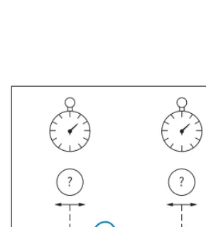
The Frequency-Time Uncertainty Relationship
We can take a different approach to uncertainty for classical waves by imagining a measurement of the period rather than the wavelength of the wave that comprises our wave packet. Suppose we have a timing device that we use to measure the duration of the wave packet, as in Figure 4.20. Here we are plotting the wave disturbance as a function of time rather than location. The “size” of the wave packet is now its duration in time, which is roughly one periodT for this wave packet, so thatt≈T. Whatever measuring device we use, we have some difficulty locating exactly the start and end of one cycle, so we have an uncertainty
T in measuring the period. As before, we’ll assume this uncertainty is some small fraction of the period:T∼εT. To examine the competition between the duration of the wave packet and our ability to measure its period, we calculate the product oftandT:
tT ∼εT2 (4.5)
? ?
∆t ≈ T
FIGURE 4.20 Measuring the period
of a wave represented by a small wave packet of duration roughly one period.
This is the second of our uncertainty relationships for classical waves. It shows that for a wave of a given period, the smaller the duration of the wave packet, the larger is the uncertainty in our measurement of the period. Note the similarity between Eqs. 4.4 and 4.5, one representing relationships in space and the other in time.
4.4 | Heisenberg Uncertainty Relationships 113
uncertainty in the frequency. Instead, they should be directly related—the better we know the period, the better we know the frequency. Here is how we obtain the relationship: Beginning withf =1/T, we take differentials on both sides:
df = − 1 T2dT
Next we convert the infinitesimal differentials to finite intervals, and because we are interested only in the magnitude of the uncertainties we can ignore the minus sign:
f = 1
T2T (4.6)
Combining Eqs. 4.5 and 4.6, we obtain
ft∼ε (4.7)
Equation 4.7 shows that the longer the duration of the wave packet, the more precisely we can measure its frequency.
Example 4.4
An electronics salesman offers to sell you a frequency-measuring device. When hooked up to a sinusoidal signal, it automatically displays the frequency of the signal, and to account for frequency variations, the frequency is remea-sured once each second and the display is updated. The salesman claims the device to be accurate to 0.01 Hz. Is this claim valid?
Solution
Based on Eq. 4.7, and again estimatingεto be about 0.1, we know that a measurement of frequency in a timet=1s
must have an associated uncertainty of about
f ∼ ε
t =
0.1 1s =0.1 Hz
It appears that the salesman may be exaggerating the precision of this device.
4.4 HEISENBERG UNCERTAINTY RELATIONSHIPS
The uncertainty relationships discussed in the previous section apply toallwaves, and we should therefore apply them to de Broglie waves. We can use the basic de Broglie relationshipp=h/λto relate the uncertainty in the momentumpto the uncertainty in wavelengthλ, using the same procedure that we used to obtain Eq. 4.6. Starting withp=h/λ, we take differentials on both sides and obtain
dp=(−h/λ2)dλ. Now we change the differentials into differences, ignoring the minus sign:
p= h
An uncertainty in the momentum of the particle is directly related to the uncertainty in the wavelength associated with the particle’s de Broglie wave packet.
Combining Eq. 4.8 with Eq. 4.4, we obtain
xp∼εh (4.9)
Just like Eq. 4.4, this equation suggests an inverse relationship betweenxand
p. The smaller the size of the wave packet of the particle, the larger is the uncertainty in its momentum (and thus in its velocity).
Quantum mechanics provides a formal procedure for calculatingxandp
for wave packets corresponding to different physical situations and for different schemes for confining a particle. One outcome of these calculations gives the wave packet with the smallest possible value of the productxp, which turns out to beh/4π, as we will discuss in the next chapter. Thusε=1/4πin this case. All other wave packets will have larger values forxp.
The combinationh/2π occurs frequently in quantum mechanics and is given the special symbol−h(“h-bar”)
− h= h
2π =1.05×10 −34
J·s=6.58×10⁻¹⁶eV·s
In terms ofh−, we can write the uncertainty relationship as
xpx 12−h (4.10) Werner Heisenberg (1901–1976,
Ger-many). Best known for the uncertainty principle, he also developed a com-plete formulation of the quantum the-ory based on matrices.
The x subscript has been added to the momentum to remind us that Eq. 4.10 applies to motion in a given direction and relates the uncertainties in position and momentum in that direction only. Similar and independent relationships can be applied in the other directions as necessary; thusypy−h/2 orzpz−h/2.
Equation 4.10 is the first of theHeisenberg uncertainty relationships. It sets the limit of the best we can possibly do in an experiment to measuresimultaneouslythe location and the momentum of a particle. Another way of interpreting this equation is to say that the more we try to confine a particle, the less we know about its momentum.
Because the limit of−h/2 represents the minimum value of the productxp
x,
in most cases we will do worse than this limit. It is therefore quite acceptable to take
xpx∼h− (4.11)
as a rough estimate of the relationship between the uncertainties in location and momentum.
Screen
y
x
a q = sin–1 la
∆x~∞
Electrons
FIGURE 4.21 Single-slit diffraction
of electrons. A wide beam of electrons is incident on a narrow slit. The elec-trons that pass through the slit acquire a component of momentum in the x
direction.
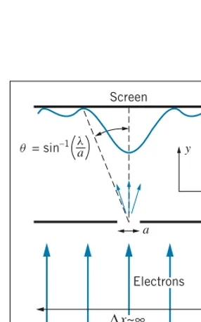
As an example, let’s consider a beam of electrons incident on a single slit, as in Figure 4.21. We know this experiment as single-slit diffraction, which produces the characteristic diffraction pattern illustrated in Figure 4.1. We’ll assume that the particles are initially moving in the y direction and that we know their momentum in that direction as precisely as possible. If the electrons initially have no component of their momentum in thexdirection, we knowpx exactly (it is exactly zero), so thatpx=0; thus we know nothing about thexcoordinates of the electrons (x=∞). This situation represents a very wide beam of electrons, only a small fraction of which pass through the slit.
4.4 | Heisenberg Uncertainty Relationships 115
in their xlocation is no larger thana, the width of the slit; thusx=a. This improvement in our knowledge of the electron’s location comes at the expense of our knowledge of its momentum, however. According to Eq. 4.11, the uncertainty in thexcomponent of its momentum is nowpx∼−h/a. Measurements beyond
the slit no longer show the particle moving precisely in the y direction (for whichpx=0); the momentum now has a smallxcomponent as well, with values distributed about zero but now with a range of roughly±−h/a. In passing through
the slit, a particle acquires on the average an x component of momentum of roughly−h/a, according to the uncertainty principle.
Let us now find the angleθthat specifies where a particle with this value ofpx
lands on the screen. For small angles, sinθ≈tanθand so
sinθ≈tanθ=px py
= − h/a
py
= λ
2πa
usingλ=h/pyfor the de Broglie wavelength of the electrons. The first minimum of the diffraction pattern of a single slit is located at sinθ=λ/a, which is larger than the spread of angles into which most of the particles are diffracted. The calculation shows that the distribution of transverse momentum given by the uncertainty principle is roughly equivalent to the spreading of the beam into the central diffraction peak, and it illustrates again the close connection between wave behavior and uncertainty in particle location.
The diffraction (spreading) of a beam following passage through a slit is just the effect of the uncertainty principle on our attempt to specify the location of the particle. As we make the slit narrower,pxincreases and the beam spreads even more. In trying to obtain more precise knowledge of the location of the particle by making the slit narrower, we have lost knowledge of the direction of its travel. This trade-off between observations of position and momentum is the essence of the Heisenberg uncertainty principle.
We can also apply the second of our classical uncertainty relationships (Eq. 4.7) to de Broglie waves. If we assume the energy-frequency relationship for light,
E=hf, can be applied to particles, then we immediately obtain E=hf. Combining this with Eq. 4.7, we obtain
Et∼εh (4.12)
Once again, the minimum uncertainty wave packet givesε=1/4π, and so
Et12h− (4.13)
This is the second of the Heisenberg uncertainty relationships. It tells us that the more precisely we try to determine the time coordinate of a particle, the less precisely we know its energy. For example, if a particle has a very short lifetime between its creation and decay (t→0), a measurement of its rest energy (and thus its mass) will be very imprecise (E→∞). Conversely, the rest energy of a stable particle (one with an infinite lifetime, so thatt=∞) can in principle be measured with unlimited precision (E=0).
As in the case of the first Heisenberg relationship, we can take
Et∼−h (4.14)
The Heisenberg uncertainty relationships are the mathematical representations of theHeisenberg uncertainty principle,which states:
It is not possible to make a simultaneous determination of the position and the momentum of a particle with unlimited precision,
and
It is not possible to make a simultaneous determination of the energy and the time coordinate of a particle with unlimited precision.
These relationships give an estimate of the minimum uncertainty that can result from any experiment; measurement of the position and momentum of a particle will give a spread of values of widthsxandpx. We may, for other reasons, do
much worse than Eqs. 4.10 and 4.13, butwe can do no better.
These relationships have a profound impact on our view of nature. It is quite acceptable to say that there is an uncertainty in locating the position of a water wave. It is quite another matter to make the same statement about a de Broglie wave, becausethere is an implied corresponding uncertainty in the position of the particle.Equations 4.10 and 4.13 say thatnature imposes a limit on the accuracy with which we can do experiments. To emphasize this point, the Heisenberg relationships are sometimes called “indeterminacy” rather than “uncertainty” principles, because the idea of uncertainty may suggest an experimental limit that can be reduced by using better equipment or technique. In actuality, these coordinates areindeterminateto the limits provided by Eqs. 4.10 and 4.13—no matter how hard we try, it is simply not possible to measure more precisely.
Example 4.5
An electron moves in the x direction with a speed of 3.6×10⁶m/s. We can measure its speed to a precision of
1%. With what precision can we simultaneously measure itsxcoordinate?
Solution
The electron’s momentum is
px=mvx=(9.11×10⁻³¹kg)(3.6×10⁶m/s)
=3.3×10⁻²⁴kg·m/s
The uncertainty px is 1% of this value, or 3.3× 10⁻²⁶kg
·m/s. The uncertainty in position is then
x∼
− h px
= 1.05 × 10 −34J
·s 3.3 ×10⁻²⁶kg·m/s
=3.2 nm
which is roughly 10 atomic diameters.
Example 4.6
Repeat the calculations of the previous example in the case of a pitched baseball (m=0.145 kg) moving at a speed of 95 mi/h (42.5 m/s). Again assume that its speed can be measured to a precision of 1%.
Solution
The baseball’s momentum is
px=mvx=(0.145 kg)(42.5 m/s)=6.16 kg·m/s
The uncertainty in momentum is 6.16×10⁻²kg
·m/s, and the corresponding uncertainty in position is
x∼
− h
px =
1.05×10⁻³⁴J
·s
6.16×10⁻²kg·m/s =1.7×10
−33
4.4 | Heisenberg Uncertainty Relationships 117
This uncertainty is 19 orders of magnitude smaller than the size of an atomic nucleus. The uncertainty principle cannot be blamed for the batter missing the pitch! Once again
we see that, because of the small magnitude of Planck’s constant, quantum effects are not observable for ordinary objects.
A Statistical Interpretation of Uncertainty
A diffraction pattern, such as that shown in Figure 4.21, is the result of the passage of many particles or photons through the slit. So far, we have been discussing the behavior of only one particle. Let’s imagine that we do an experiment in which a large number of particles passes (one at a time) through the slit, and we measure the transverse (x component) momentum of each particle after it passes through the slit. We can do this experiment simply by placing a detector at different locations on the screen where we observe the diffraction pattern. Because the detector actually accepts particles over a finite region on the screen, it measures in a range of deflection angles or equivalently in a range of transverse momentum. The result of the experiment might look something like Figure 4.22. The vertical scale shows the number of particles with momentum in each interval corresponding to different locations of the detector on the screen. The values are symmetrically arranged about zero, which indicates that the mean or average value of px is zero. Thewidth of the distribution is characterized bypx.
Momentum 0
∆p x
Number of particles recorded by detector
FIGURE 4.22 Results that might be
obtained from measuring the number of electrons in a given time interval at different locations on the screen of Figure 4.21. The distribution is cen-tered aroundpx=0 and has a width
that is characterized bypx. Figure 4.22 resembles a statistical distribution, and in fact the precise definition
ofpx is similar to that of the standard deviationσAof a quantityAthat has a
mean or average valueAav:
σA=
(A2)
av−(Aav)2
If there areN individual measurements ofA, thenAav=N−1Aiand(A2)av= N−1A2i.
By analogy, we can make a rigorous definition of the uncertainty in momentum as
px=(p2
x)av−(px,av)2 (4.15)
The average value of the transverse momentum for the situation shown in Figure 4.22 is zero, so
px=
(p2
x)av (4.16)
which gives in effect a root-mean-square value ofpx. This can be taken to be a rough measure of the magnitude ofpx. Thus it is often said thatpx gives a measure of the magnitude of the momentum of the particle. As you can see from Figure 4.22, this is indeed true.∗
∗The relationship between the value ofp
xcalculated from Eq. 4.16 and the width of the distribution
Example 4.7
In nuclear beta decay, electrons are observed to be ejected from the atomic nucleus. Suppose we assume that elec-trons are somehow trapped within the nucleus, and that occasionally one escapes and is observed in the laboratory. Take the diameter of a typical nucleus to be 1.0×10⁻¹⁴m, and use the uncertainty principle to estimate the range of kinetic energies that such an electron must have.
Solution
If the electron were trapped in a region of width x≈ 10−14m, the corresponding uncertainty in its momentum
would be
momentum is clearly in the relativistic regime for electrons, so we must use the relativistic formula to find the kinetic
energy for a particle of momentum 19.7 MeV/c:
K=p2c2+(mc2)2−mc2
=(19.7 MeV)2+(0.5 MeV)2−0.5 MeV=19 MeV
where we have used Eq. 4.16 to relate px to p2x. This
result gives the spread of kinetic energies corresponding to a spread in momentum of 19.7 MeV/c.
Electrons emitted from the nucleus in nuclear beta decay typically have kinetic energies of about 1 MeV, much smaller than the typical spread in energy required by the uncertainty principle for electrons confined inside the nucleus. This suggests that beta-decay electrons of such low energies cannot be confined in a region of the size of the nucleus, and that another explanation must be found for the electrons observed in nuclear beta decay. (As we discuss in Chapter 12, these electrons cannot preexist in the nucleus, which would violate the uncertainty principle, but are “manufactured” by the nucleus at the instant of the decay.)
Example 4.8
(a) A charged pi meson has a rest energy of 140 MeV and a lifetime of 26 ns. Find the energy uncertainty of the pi meson, expressed in MeV and also as a fraction of its rest energy. (b) Repeat for the uncharged pi meson, with a rest energy of 135 MeV and a lifetime of 8.3×10⁻¹⁷s.
(c) Repeat for the rho meson, with a rest energy of 765 MeV and a lifetime of 4.4×10⁻²⁴s.
Solution
(a) If the pi meson lives for 26 ns, we have only that much time in which to measure its rest energy, and Eq. 4.8 tells us thatanyenergy measurement done in a timetis uncertain by an amount of at least
E=
In the first case, the uncertainty principle does not give a large enough effect to be measured—particle masses cannot be measured to a precision of 10−16 (about 10−6
4.5 | Wave Packets 119
instruments and therefore might be observable in the lab-oratory. In the third example, we see that the uncertainty principle can contribute substantially to the precision of our knowledge of the rest energy of the rho meson; measure-ments of its rest energy will show a statistical distribution centered about 765 MeV with a spread of 150 MeV, and no matter how precise an instrument we use to measure the rest energy, we can never reduce that spread.
The lifetime of a very short-lived particle such as the rho meson cannot be measured directly. In practice we reverse the procedure of the calculation of this example— we measure the rest energy, which gives a distribution similar to Figure 4.22, and from the “width”Eof the distribution we deduce the lifetime using Eq. 4.8. This procedure is discussed in Chapter 14.
Example 4.9
Estimate the minimum velocity that would be measured for a billiard ball (m≈100 g) confined to a billiard table of dimension 1 m.
Solution
Forx≈1 m, we have
px∼ − h
x=
1.05×10⁻³⁴J·s
1 m =1×10 −34kg
·m/s so
vx=
px
m =
1×10⁻³⁴kg
·m/s
0.1 kg =1×10 −33m/s
Thus quantum effects might result in motion of the billiard ball with a speed distribution having a spread of about 1× 10⁻³³m/s. At this speed, the ball would move a distance
of 1% of the diameter of an atomic nucleus in a time equal to the age of the universe! Once again, we see that quantum effects are not observable with macroscopic objects.
4.5 WAVE PACKETS
In Section 4.3, we described measurements of the wavelength or frequency of a wave packet, which we consider to be a finite group of oscillations of a wave. That is, the wave amplitude is large over a finite region of space or time and is very small outside that region.
Before we begin our discussion, it is necessary to keep in mind that we are discussingtraveling waves, which we imagine as moving in one direction with a uniform speed. (We’ll discuss the speed of the wave packet later.) As the wave packet moves, individual locations in space will oscillate with the frequency or wavelength that characterizes the wave packet. When we show a static picture of a wave packet, it doesn’t matter that some points within the packet appear to have positive displacement, some have negative displacement, and some may even have zero displacement. As the wave travels, those locations are in the process of oscillating, and our drawings may “freeze” that oscillation. What is important is the locations in space where the overall wave packet has a large oscillation amplitude and where it has a very small amplitude.∗
In this section we will examine how to build a wave packet by adding waves together. A pure sinusoidal wave is of no use in representing a particle—the wave
∗By analogy, think of a radio wave traveling from the station to your receiver. At a particular instant
extends from−∞to+∞, so the particle could be found anywhere. We would like the particle to be represented by a wave packet that describes how the particle is
localizedto a particular region of space, such as an atom or a nucleus.
The key to the process of building a wave packet involves adding together waves of different wavelength. We represent our waves asAcoskx, wherekis the wave number (k=2π/λ) andAis the amplitude. For example, let’s add together two waves:
y(x)=A1cosk1x+A2cosk2x=A1cos(2πx/λ1)+A2cos(2πx/λ2) (4.17)
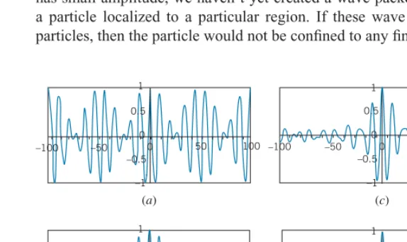
This sum is illustrated in Figure 4.23afor the caseA1=A2andλ1=9,λ2=11. This combined wave shows the phenomenon known asbeatsin the case of sound waves. So far we don’t have a result that looks anything like the wave packet we are after, but you can see that by adding together two different waves we have reduced the amplitude of the wave packet at some locations. This pattern repeats endlessly from−∞to+∞, so the particle is still not localized.
Let’s try a more detailed sum. Figure 4.23bshows the result of adding 5 waves with wavelengths 9, 9.5, 10, 10.5, 11. Here we have been a bit more successful in restricting the amplitude of the wave packet in some regions. By adding even more waves with a larger range of wavelengths, we can obtain still narrower regions of large amplitude: Figure 4.23c shows the result of adding 9 waves with wavelengths 8, 8.5, 9,. . ., 12, and Figure 4.23d shows the result of adding 13 waves of wavelengths 7, 7.5, 8,. . ., 13. Unfortunately, all of these patterns (including the regions of large amplitude) repeat endlessly from−∞to+∞, so even though we have obtained increasingly large regions where the wave packet has small amplitude, we haven’t yet created a wave packet that might represent a particle localized to a particular region. If these wave packets did represent particles, then the particle would not be confined to any finite region.
–100 –50 –0.5
–1 (a) 0.5
0
0 50 100
1
1
–100 –50 –0.5
50 100
(b)
0 0 0.5
–1
(c) –100 –50
–0.5
–1
0 50
1
100 0.5
0
(d)
–100 –50 –0.5
–1
0 50
1
100 0.5
0
FIGURE 4.23 (a) Adding two waves of wavelengths 9 and 11 gives beats.
4.5 | Wave Packets 121
The regions of large amplitude in Figures 4.23b,c,ddo show how adding more waves of a greater range of wavelengths helps to restrict the size of the wave packet. The region of large amplitude in Figure 4.23branges from aboutx= −40 to+40, while in Figure 4.23cit is from aboutx= −20 to+20 and in Figure 4.23d
from aboutx= −15 to+15. This shows again the inverse relationship betweenx
andλexpected for wave packets given by Eq. 4.4: as the range of wavelengths increases from 2 to 4 to 6, the size of the “allowed” regions decreases from about 80 to 40 to 30. Once again we find that to restrict the size of the wave packet we must sacrifice the precise knowledge of the wavelength.
Note that for all four of these wave patterns, the disturbance seems to have a wavelength of about 10, equal to the central wavelength of the range of values of the functions we constructed. We can therefore regard these functions as a cosine wave with a wavelength of 10 that is shaped ormodulated by the other cosine waves included in the function. For example, for the case ofA1=A2=A, Eq. 4.17 can be rewritten after a bit of trigonometric manipulation as
y(x)=2Acos with a wavelength of 10, and the first cosine term provides the shaping envelope that produces the beats. in which the modulation envelope decreases in amplitude like 1/x. (b) A wave packet with a Gaussian modulating function. Both curves are drawn for λ0=10 and λ=0.58,
which corresponds approximately to Figure 4.23b.
Any finite combination of waves with discrete wavelengths will produce patterns that repeat between−∞ to+∞, so this method of adding waves will not work in constructing a finite wave packet. To construct a wave packet with a finite width, we must replace the first cosine term in Eq. 4.19 with a function that is large in the region where we want to confine the particle but that falls to zero asx→ ±∞. For example, the simplest function that has this property is 1/x, so we might imagine a wave packet whose mathematical form is
y(x)= 2A
Hereλ0represents the central wavelength, replacingλav. (In going from Eq. 4.19 to Eq. 4.20, the cosine modulating term has been changed to a sine; otherwise the function would blow up atx=0.) This function is plotted in Figure 4.24a. It looks more like the kind of function we are seeking—it has large amplitude only in a small region of space, and the amplitude drops rapidly to zero outside that region. Another function that has this property is theGaussianmodulating function:
y(x)=Ae−2(λπx/λ20)2cos
Both of these functions show the characteristic inverse relationship between an arbitrarily defined size of the wave packetxand the wavelength range parameter
λthat is used in constructing the wave packet. For example, consider the wave packet shown in Figure 4.24a. Let’s arbitrarily define the width of the wave packet as the distance over which the amplitude of the central region falls by 1/2. That occurs roughly where the argument of the sine has the value±π/2, which gives
xλ∼λ20, consistent with our classical uncertainty estimate.
These wave packets can also be constructed by adding together waves of differing amplitude and wavelength, but the wavelengths form a continuous rather than a discrete set. It is a bit easier to illustrate this if we work with wave number
k=2π/λrather than wavelength. So far we have been adding waves in the form ofAcoskx, so that
y(x)=Aicoskix (4.22)
whereki=2π/λi. The waves plotted in Figure 4.23 represent applications of the general formula of Eq. 4.22 carried out over different numbers of discrete waves. If we have a continuous set of wave numbers, the sum in Eq. 4.22 becomes an integral:
y(x)=
A(k)coskx dk (4.23)
where the integral is carried out over whatever range of wave numbers is permitted (possibly infinite).
For example, suppose we have a range of wave numbers fromk0−k/2 to k0+k/2 that is a continuous distribution of wave numbers of widthkcentered atk0. If all of the waves have the same amplitudeA0, then from Eq. 4.23 the form of the wave packet can be shown to be (see Problem 24 at the end of the chapter)
y(x)= 2A0 x sin
k
2 x
cosk0x (4.24)
This is identical with Eq. 4.20 with k0=2π/λ0 and k=2π λ/λ20. This
relationship betweenkandλfollows from a procedure similar to what was used to obtain Eq. 4.6. Withk=2π/λ, taking differentials givesdk= −(2π/λ2)dλ. Replacing the differentials with differences and ignoring the minus sign gives the relationship betweenkandλ.
A better approximation of the shape of the wave packet can be found by letting
A(k)vary according to a Gaussian distribution A(k)=A0e−(k−k0)2/2(k)2. This
gives a range of wave numbers that has its largest contribution at the central wave numberk0 and falls off to zero for larger or smaller wave numbers with a characteristic width ofk. Applying Eq. 4.23 to this case, withkranging from −∞to+∞gives (see Problem 25)
y(x)=A0k√2πe−(kx)2/2cosk0x (4.25)
which shows how the form of Eq. 4.21 originates.
4.6 | The Motion of a Wave Packet 123
of widthxwill have a distribution of wavelengths characterized by a widthλ. The smaller we try to makex, the larger will be the spreadλof the wavelength distribution. The mathematics of this process gives a result that is consistent with the uncertainty relationship for classical waves (Eq. 4.4).
4.6 THE MOTION OF A WAVE PACKET
Let’s consider again the “beats” wave packet represented by Eq. 4.17 and illustrated in Figure 4.23a. We now want to turn our “static” waves into traveling waves. It will again be more convenient for this discussion to work with the wave numberkinstead of the wavelength. To turn a static wavey(x)=Acoskxinto a traveling wave moving in the positivexdirection, we replacekxwithkx−ωt, so that the traveling wave is written asy(x,t)=Acos(kx−ωt). (For motion in the negativexdirection, we would replacekxwithkx+ωt.) Hereωis thecircular frequencyof the wave:ω=2πf. The combined traveling wave then would be represented as
y(x,t)=A1cos(k1x−ω1t)+A2cos(k2x−ω2t) (4.26)
For any individual wave, the wave speed is related to its frequency and wavelength according tov=λf. In terms of the wave number and circular frequency, we can write this asv=(2π/k)(ω/2π ), sov=ω/k. This quantity is sometimes called thephase speedand represents the speed of one particular phase or component of the wave packet. In general, each individual component may have a different phase speed. As a result, the shape of the wave packet may change with time.
For Figure 4.23a, we choseA1 =A2andλ1=9,λ2=11. Let’s choosev1 =6 units/s andv2=4 units/s. Figure 4.25 shows the waveform at a time oft=1 s. In that time, wave 1 will have moved a distance of 6 units in the positivexdirection and wave 2 will have moved a distance of 4 units in the positive xdirection. However, the combined wave moves a much greater distance in that time: the center of the beat that was formerly atx=0 has moved tox=15 units. How is it possible that the combined waveform moves faster than either of its component waves?
–100 –50
–0.5
–1 0.5
1
50 100
0 0
FIGURE 4.25 The solid line shows the waveform of Figure 4.23a
To produce the peak atx=0 andt=0, the two component waves were exactly in phase—their two maxima lined up exactly to produce the combined maximum of the wave. At x=15 units and t=1 s, two individual maxima line up once again to produce a combined maximum. They arenotthe same two maxima that lined up to produce the maximum att=0, but it happens that two other maxima are in phase atx=15 units andt=1 s to produce the combined maximum. If we were to watch an animation of the wave, we would see the maximum originally atx=0 move gradually tox=15 betweent=0 andt=1 s.
We can understand how this occurs by writing Eq. 4.26 in a form similar to Eq. 4.18 using trigonometric identities. The result is (again assumingA1=A2 = A, as we did in Eq. 4.18):
As in Eq. 4.18, the second term in Eq. 4.27 represents the rapid variation of the wave within the envelope given by the first term. It is the first term that dictates the overall shape of the waveform, so it is this term that determines the speed of travel of the waveform. For a wave that is written as cos(kx−ωt), the speed isω/k. For this wave envelope, the speed is(ω/2)/(k/2)=ω/k. This speed is called the group speed of the wave packet. As we have seen, the group speed of the wave packet can be very different from the phase speed of the component waves. For more complicated situations than the two-component “beat” waveform, the group speed can be generalized by turning the differences into differentials:
vgroup= dω
dk (4.28)
The group speed depends on the relationship between frequency and wavelength for the component waves. If the phase speed of all component waves is the same and is independent of frequency or wavelength (as, for example, light waves in empty space), then the group speed is identical to the phase speed and the wave packet keeps its original shape as it travels. In general, the propagation of a component wave depends on the properties of the medium, and different component waves will travel with different speeds. Light waves in glass or sound waves in most solids travel with a speed that varies with frequency or wavelength, and so their wave packets change shape as they travel. De Broglie waves in general have different phase speeds, so that their wave packets expand as they travel.
Example 4.10
Certain ocean waves travel with a phase velocityvphase=
gλ/2π, wheregis the acceleration due to gravity. What is the group velocity of a “wave packet” of these waves?
Solution
4.6 | The Motion of a Wave Packet 125
The Group Speed of deBroglie Waves
Suppose we have a localized particle, represented by a group of de Broglie waves. For each component wave, the energy of the particle is related to the frequency of the de Broglie wave byE=hf =−hω, and sodE
=−hdω. Similarly, the momentum of the particle is related to the wavelength of the de Broglie wave byp=h/λ=−hk, sodp=−hdk. The group speed of the de Broglie wave then can
be expressed as
vgroup= dω dk =
dE/−h dp/−h =
dE
dp (4.29)
For a classical particle having only kinetic energyE=K=p2/2m, we can find dE/dpas
dE dp =
d dp
p2
2m
= p
m =v (4.30)
which is the velocity of the particle.
Combining Eqs. 4.29 and 4.30 we obtain an important result:
vgroup=vparticle (4.31)
The speed of a particle is equal to the group speed of the corresponding wave packet.The wave packet and the particle move together—wherever the particle goes, its de Broglie wave packet moves along with it like a shadow. If we do a wave-type experiment on the particle, the de Broglie wave packet is always there to reveal the wave behavior of the particle. A particle can never escape its wave nature!
The Spreading of a Moving Wave Packet
Suppose we have a wave packet that represents a confined particle att=0. For example, the particle might have passed through a single-slit apparatus. Its initial uncertainty in position isx0 and its initial uncertainty in momentum ispx0. The wave packet moves in thexdirection with velocityvx, but that velocity is not precisely known—the uncertainty in its momentum gives a corresponding uncertainty in velocity:vx0 =px0/m. Because there is an uncertainty in the velocity of the wave packet, we can’t be sure where it will be located at time
t. That is, its location at timet isx=vxt, with velocityvx=vx0±vx0. Thus there are two contributions to the uncertainty in its location at timet: the initial uncertainty x0 and an additional amount equal to vx0t that represents the
spreading of the wave packet. We’ll assume that these two contributions add quadratically, like experimental uncertainties, so that the total uncertainty in the location of the particle is
x=
(x0)2+(vx0t)2=
(x0)2+(px0t/m)2 (4.32)
Takingpx0=−h/x
0according to the uncertainty principle, we have
x=
(x0)2+(−ht/mx
0)2 (4.33)
If we try to make the wave packet very small att=0 (x0is small), then the second
term under the square root makes the wave packet expand rapidly, becausex0