A New Three Object Triangulation Algorithm for
Mobile Robot Positioning
Vincent Pierlot
, Member, IEEE
, and Marc Van Droogenbroeck
, Member, IEEE
Abstract—Positioning is a fundamental issue in mobile robot
applications. It can be achieved in many ways. Among them, tri-angulation based on angles measured with the help of beacons is a proven technique. Most of the many triangulation algorithms proposed so far have major limitations. For example, some of them need a particular beacon ordering, have blind spots, or only work within the triangle defined by the three beacons. More reliable methods exist; however, they have an increasing complexity, or they require to handle certain spatial arrangements separately. In this paper, we present a simple and new three object triangula-tion algorithm, known as ToTal, that natively works in the whole plane and for any beacon ordering. We also provide a compre-hensive comparison between many algorithms and show that our algorithm is faster and simpler than comparable algorithms. In addition to its inherent efficiency, our algorithm provides a very useful and unique reliability measure that is assessable anywhere in the plane, which can be used to identify pathological cases, or as a validation gate in Kalman filters.
Index Terms—Mobile robot, positioning, triangulation.
I. INTRODUCTION
P
OSITIONING is a fundamental issue in mobile robot ap-plications. Indeed, in most cases, a mobile robot that moves in its environment has to position itself before it can execute its actions properly. Therefore, the robot has to be equipped with some hardware and software capable to provide a sensory feed-back related to its environment [3]. Positioning methods can be classified into two main groups [5]: (1) relative position-ing (also calleddead-reckoning) and (2)absolute positioning (or reference-based). One of the most famous relative position-ing technique is the odometry, which consists of countposition-ing the number of wheel revolutions to compute the offset relative to a known position. It is very accurate for small offsets but is not sufficient because of the unbounded accumulation of errors over time (because of wheel slippage, imprecision in the wheel cir-cumference, or wheel base) [5]. Furthermore, odometry needs an initial position and fails when the robot is “waken-up” (after a forced reset for example) or is raised and dropped somewhere, since the reference position is unknown or modified. Anabso-Manuscript received April 5, 2013; revised September 27, 2013; accepted December 2, 2013. Date of publication January 2, 2014; date of current version June 3, 2014. This paper was recommended for publication by Associate Editor P. Jensfelt and Editor D. Fox upon evaluation of the reviewers’ comments.
The authors are with the INTELSIG, Laboratory for Signal and Image Ex-ploitation, Montefiore Institute, University of Li`ege, Li`ege, Belgium (e-mail: [email protected]; [email protected]).
Color versions of one or more of the figures in this paper are available online at http://ieeexplore.ieee.org.
Digital Object Identifier 10.1109/TRO.2013.2294061
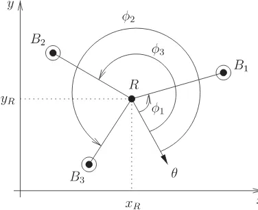
Fig. 1. Triangulation setup in the 2-D plane.Rdenotes the robot.B1,B2,
andB3 are the beacons.φ1,φ2, andφ3 are the angles forB1,B2, andB3,
respectively, relative to the robot reference orientationθ. These angles may be used by a triangulation algorithm in order to compute the robot position
{xR, yR}and orientationθ.
lute positioning system is thus required to recalibrate the robot position periodically.
Relative and absolute positioning are complementary to each other [3], [6] and are typically merged together by using a Kalman filter [17], [21]. In many cases, absolute positioning is ensured by beacon-based triangulation or trilateration. Triangu-lationis the process of determining the robot pose (position and orientation) based on angle measurements, whiletrilateration
methods involve the determination of the robot position based on distance measurements. Because of the availability of angle measurement systems, triangulation has emerged as a widely used, robust, accurate, and flexible technique [14]. Another ad-vantage of triangulation versus trilateration is that the robot can compute its orientation (or heading) in addition to its position so that the completeposeof the robot can be found. The pro-cess to determine the robot pose based on angle measurements is generally termed triangulation. The word triangulation is a wide concept, which does not specify if the angles are measured from the robot or the beacons, nor the number of angles used. In this paper, we are interested in self position determination, meaning that the angles are measured from the robot location. Fig. 1 illustrates our triangulation setup.
Moreover, if only three beacons are used in self position determination, triangulation is also termedThree Object Trian-gulationby Cohen and Koss [10]. Here, the general termobject
refers to a 2-D point, whose location is known.
Our algorithm, which will be known as ToTal1hereafter, has already been presented in a previous paper [33]. In this paper, we
1ToTal stands for:ThreeobjectTriangulationalgorithm.
supplement our previous work with an extensive review about the triangulation topics, detail the implementation of our algo-rithm, and compare our algorithm with seventeen other similar algorithms. Please note that the C source code implementation, developed for the error analysis and benchmarks, is made avail-able to the scientific community.
The paper is organized as follows. Section II reviews some of the numerous triangulation algorithms found in the literature. Our new three object triangulation algorithm is described in Section III. Section IV presents simulation results and bench-marks. Then, we conclude the paper in Section V.
II. RELATEDWORK
A. Triangulation Algorithms
The principle of triangulation has existed for a long time, and many methods have been proposed so far. One of the first comprehensive reviewing work has been carried out by Co-hen and Koss [10]. In their paper, they classify the triangula-tion algorithms into four groups: (1)Geometric Triangulation, (2)Geometric Circle Intersection, (3)Iterative methods (Itera-tive Search, Newton–Raphson, etc.), and (4)Multiple Beacons Triangulation.
The first group could be namedTrigonometric Triangulation,
because it makes an intensive use of trigonometric functions. Al-gorithms of the second group determine the parameters (radius and center) of two (of the three) circles that pass through the bea-cons and the robot, then they compute the intersection between these two circles. Methods of the first and second groups are typically used to solve the three object triangulation problem. The third group linearizes the trigonometric relations to con-verge to the robot position after some iterations, from a starting point (usually the last known robot position). In the iterative methods, they also presentIterative Search, which consists in searching the robot position through the possible space of ori-entations, and by using a closeness measure of a solution. The fourth group addresses the more general problem of finding the robot pose from more than three angle measurements (usually corrupted by errors), which is an overdetermined problem.
Several authors have noticed that the second group ( Geomet-ric Circle Intersection) is the most popular to solve the three object triangulation problem [18], [31]. The oldest Geometric Circle Intersection algorithm was described by McGillem and Rappaport [30], [31]. Font-Llagunes and Battle [18] present a very similar method, however they first change the reference frame to relocate beacon 2 at the origin and beacon 3 on theX -axis. They compute the robot position in this reference frame and then, they apply a rotation and translation to return to the origi-nal reference frame. Zalamaet al.[45], [46] present a hardware system to measure angles to beacons and a method to compute the robot pose from three angle measurements. A similar hard-ware system and method based on [45] and [46] is described by Tsukiyama [44]. Kortenkamp [23] presents a method which turns out to be exactly the same as the one described by Cohen and Koss [10]. All these methods compute the intersection of two of the three circles that pass through the beacons and the robot. It appears that they are all variations or improvements
of older methods of McGillem and Rappaport, or Cohen and Koss. The last one is described by Lukicet al.[8], [27], but it is not general, as it only works for a subset of all possible beacon locations.
Some newer variations of Geometric/Trigonometric triangu-lation algorithms are also described in the literature. In [14], Es-teveset al.extend the algorithm presented earlier by Cohen and Koss [10] to work for any beacon ordering and to work outside the triangle formed by the three beacons. In [15] and [16], they describe the improved version of their algorithm to handle the remaining special cases (when the robot lies on the line that joins the two beacons). They also analyze the position and orienta-tion error sensitivity in [16]. Whereas Easton and Cameron [12] concentrate on an error model for the three object triangulation problem, they also briefly present an algorithm that belongs to this family. Their simple method works in the whole plane and for any beacon ordering. The work of Hmam [20] is based on Esteveset al., as well as Cohen and Koss. He presents a method, valid for any beacon ordering, that divides the whole plane into seven regions and handles two specific configurations of the robot relatively to the beacons. In [28], Madsen and Andersen describe a vision-based positioning system. Such an algorithm belongs to the trigonometric triangulation family as the vision system is used to measure angles between beacons.
However, Ligas intersects one radical axis and one circle, whereas our algorithm intersects the three radical axes of the three pairs of circles.2 Likewise, Ligas also uses only two trigonometric functions (like our method ToTal), and as a con-sequence, it is one of the most efficient methods (with ToTal), as shown in Section IV-B.
Some of the Multiple Beacons Triangulation (multiangula-tion) algorithms are described hereafter. One of the first work in this field was presented by Avis and Imai [1]. In their method, the robot measureskangles from a subset ofn indistinguish-able landmarks, and therefore they produce a bounded set a valid placements of the robot. Their algorithm runs inO(kn2)if the
robot has a compass or inO(kn3)otherwise. The most famous
algorithm was introduced by Betke and Gurvits [3]. They use an efficient representation of landmark 2-D locations by complex numbers to compute the robot pose. The landmarks are sup-posed to have an identifier known by the algorithm. The authors show that the complexity of their algorithm is proportional to the number of beacons. They also performed experiments with noisy angle measurements to validate their algorithm. Finally, they explain how the algorithm deals with outliers. Another in-teresting approach is proposed by Shimshoni [36]. He presents an efficient SVD based multiangulation algorithm from noisy angle measurements and explains why transformations have to be applied to the linear system in order to improve the accuracy of the solution. The solution is very close to the optimal solution computed with nonlinear optimization techniques, while being more than a hundred times faster. Briechle and Hanebeck [7] present a new localization approach in the case of relative bear-ing measurements by reformulatbear-ing the given localization prob-lem as a nonlinear filtering probprob-lem.
Siadat and Vialle [38] describe a multiangulation method based on the Newton–Raphson iterative method to converge to a solution minimizing an evaluation criterion. Lee et al.
[24] present another iterative method very similar to Newton– Raphson. Their algorithm was first designed to work with three beacons, however it can also be generalized to a higher number of beacons. The initial point of the convergence process is set to the center of the beacons, and good results are obtained after only four steps.
Sobreira et al. [41] present a hybrid triangulation method working with two beacons only. They use a concept similar to the
running-fixmethod introduced by Bais in [2], in which the robot has to move by a known distance to create a virtual beacon mea-surement and to compute the robot pose after it has stopped to take another angle measurement. In [40], Sobreiraet al.perform an error analysis of their positioning system. In particular, they express the position uncertainty originated by errors on mea-sured angles in terms of a surface. Sanchizet al.[35] describe another multiangulation method based onIterative Searchand circular correlation. They first compute the robot orientation by maximizing the circular correlation between the expected bea-cons angles and the measured beabea-cons angles. Then, a method similar toIterative Searchis applied to compute the position. Hu and Gu [21] present a multiangulation method based on
2Note that the paper of Ligas [25] is posterior to ours [33].
Kohonen neural network to compute the robot pose and to initialize an extended Kalman filter used for navigation.
B. Brief Discussion
It is difficult to compare all the above mentioned algorithms, because they operate in different conditions and have distinct behaviors. In practice, the choice is dictated by the application requirements and some compromises. For example, if the setup contains three beacons only or if the robot has limited on-board processing capabilities, methods of the first and second groups are the best candidates. Methods of the third and fourth groups are appropriate if the application must handle multiple beacons and if it can accommodate a higher computational cost. The main drawback of the third group is the convergence issue (existence or uniqueness of the solution) [10]. The main drawback of the fourth group is the computational cost [3], [7], [36].
The drawbacks of the first and second group are usually a lack of precision related to the following elements: 1) The beacon ordering needed to get the correct solution, 2) the consistency of the methods when the robot is located outside the triangle de-fined by the three beacons, 3) the strategy to follow when falling into some particular geometrical cases (that induce mathemat-ical underdeterminations when computing trigonometric func-tions with arguments like0orπ, division by0, etc.), and 4) the reliability measure of the computed position. Simple methods of the first and second groups usually fail to propose a proper answer to all of these concerns. For example, to work in the en-tire plane and for any beacon ordering (for instance [16]), they have to consider a set of special geometrical cases separately, that results in a lack of clarity. Finally, to our knowledge, none of these algorithms gives a realistic reliability measure of the computed position.
C. Other Aspects of Triangulation
For now, we have focused on the description of triangulation algorithms which are used to compute the position and orien-tation of the robot. Other aspects of triangulation have to be considered as well to achieve an optimal result on the robot pose in a practical situation. These are: 1) the sensitivity anal-ysis of the triangulation algorithm, 2) the optimal placement of the landmarks, 3) the selection of some landmarks among the available ones to compute the robot pose, and 4) the knowledge of the true landmark locations in the world and the true location of the angular sensor on the robot.
Optimal landmark placement has been extensively studied. Sinriech and Shoval [37], [39] define a nonlinear optimization model used to determine the position of the minimum number of beacons required by a shop floor to guarantee an accurate and reliable performance for automated guided vehicles. De-maineet al.[11] present a polynomial time algorithm to place reflector landmarks such that the robot can always localize itself from any position in the environment, which is represented by a polygonal map. Tedkas and Isler [42], [43] address the problem of computing the minimum number and placement of sensors so that the localization uncertainty at every point in the workspace is less than a given threshold. They use the uncertainty model for angle based positioning derived by Kelly [22].
Optimal landmark selection has been studied by Madsen
et al.[28], [29]. They propose an algorithm to select the best triplet among several landmarks seen by a camera, that yields to the best position estimate. The algorithm is based on a “good-ness” measure derived from an error analysis which depends on landmarks and on the robot relative pose.
To have a good sensor that provides precise angle measure-ments as well as a good triangulation algorithm is not the only concern to get accurate positioning results. Indeed, the angle sensor could be subject to nonlinearities in the measuring angle range (a complete revolution). Moreover, the beacon locations that are generally measured manually are subject to inaccura-cies, which affect directly the positioning algorithm. In their pa-per, Loevsky and Shimshoni [26] propose a method to calibrate the sensor and a method to correct the measured beacon loca-tions. They show that their procedure is effective and mandatory to achieve good positioning performance.
In the remainder of this paper, we concentrate on three object triangulation methods. Our paper presents a new three object triangulation algorithm that works in the entire plane (except when the beacons and the robot are concyclic or collinear), and for any beacon ordering. Moreover, it minimizes the number of trigonometric computations and provides a unique quantitative reliability measure of the computed position.
III. DESCRIPTION OF ANEWTHREEOBJECT TRIANGULATIONALGORITHM
Our motivation for a new triangulation algorithm is fourfold: 1) We want it to be independent of the beacon ordering, 2) the algorithm must also be independent of the relative positions of the robot and the beacons, 3) the algorithm must be fast and simple to implement in a dedicated processor, and 4) the algorithm has to provide a criterion to qualify the reliability of the computed position.
Our algorithm, named, ToTal, belongs to the family of Geo-metric Circle Intersectionalgorithms (that is, the second group). It first computes the parameters of the three circles that pass through the robot and the three pairs of beacons. Then, it com-putes the intersection of these three circles, by using all the three circles parameters (not only two of them, to the contrary of other methods).
Our algorithm relies on two assumptions: 1) The beacons are distinguishable (a measured angle can be associated to a given beacon); and (2) the angle measurements from the
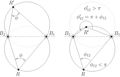
bea-Fig. 2. (Left) Locus of pointsRthatseetwo fixed pointsB1 andB2 with
a constant angleγ, in the 2-D plane, is formed by two arcs of circle. (Right) Ambiguity is removed by taking the following convention:φ1 2=φ2−φ1.
cons are taken separately, and relatively to some reference angle θ, usually the robot heading (see Fig. 1). Note that the second hy-pothesis simply states that angles are given by a rotating angular sensor. Such sensors are common in mobile robot positioning that uses triangulation [4], [5], [24], [31], [32], [45]. By con-vention, in the following, we consider that angles are measured counterclockwise (CCW), like angles on the trigonometric cir-cle. To invert the rotating direction to clockwise (CW) would only require minimal changes of our algorithm.
A. First Part of the Algorithm: The Circle Parameters
In a first step, we want to calculate the locus of the robot positions R, that see two fixed beacons, B1 and B2, with a
constant angleγ, in the 2-D plane. It is a well-known result that this locus is an arc of the circle that passes throughB1 andB2,
whose radius depends on the distance betweenB1andB2, and
γ(Proposition 21 of Book III of Euclid’s Elements [48]). More precisely, this locus is composed of two arcs of circle, which are the reflection of each other through the line that joins B1 and
B2(see the continuous lines on the left-hand side of Fig. 2).
A robot that measures an angleγbetween two beacons can stand on either of these two arcs. This case occurs if the beacons are not distinguishable or if the angular sensor is not capable to measure angles larger than π(like a vision system with a limited field of view, as used by Madsenet al.[28]). To avoid this ambiguity, we impose that, as shown on the right-hand side of Fig. 2, the measured angle between two beacons B1
andB2, which is denoted φ12, is always computed as φ12=
φ2−φ1 (this choice is natural for a CCW rotating sensor).
This is consistent with our measurement considerations, and it removes the ambiguity about the locus; however, it requires that beacons are indexed and that the robot is capable to establish the index of any beacon. As a result, the locus is a single circle that passes throughR,B1, andB2. In addition, the line joiningB1
andB2 divides the circle into two parts: one forφ12 < πand
the other forφ12 > π. In the following, we compute the circle
parameters.
expressing angles as the argument of complex numbers. In par-ticular, the angle of(B2−R)is equal to that of(B1−R)plus
φ12. Equivalently
arg
B
2−R
B1−R
=φ12 (1)
⇒arg(B2−R) (B1−R)
=φ12. (2)
Then, if we substitute R, B1, B2, respectively by (x+iy), (x1+iy1),(x2+iy2), we have that
arg
(x2+iy2−x−iy) (x1−iy1−x+iy)e−iφ1 2= 0
(3)
⇒ −sinφ12(x2−x) (x1−x) + sinφ12(y2−y) (y−y1) + cosφ12(x2−x) (y−y1) + cosφ12(y2−y) (x1−x) = 0
(4)
wherei=√−1. After lengthy simplifications, we find the locus
(x−x12)2+ (y−y12)2 =R212 (5)
which is a circle whose center{x12, y12}is located at
x12 = (x1+x2) + cotφ12(y1−y2)
2 (6)
y12 =
(y1+y2)−cotφ12(x1−x2)
2 (7)
and whose squared radius equals
R212 =
(x1−x2)2+ (y1−y2)2 4 sin2φ12
. (8)
The three last equations may also be found in [18]. The replace-ment ofφ12byπ+φ12 in the above equations yields the same
circle parameters (see the right-hand side of Fig. 2), which is consistent with our measurement considerations. For an angular sensor that turns in the CW direction, these equations are iden-tical except that one has to change the sign ofcot(.)in (6) and (7).
Hereafter, we use the following notations:
1) Biis the beaconi, whose coordinates are{xi, yi}.
2) Ris the robot position, whose coordinates are{xR, yR}.
3) φiis the angle for beaconBi.
4) φij =φj−φi is the bearing angle between beaconsBi
andBj.
5) Tij = cot(φij).
6) Cij is the circle that passes throughBi,Bj, andR.
7) cijis the center ofCij, whose coordinates are{xij, yij}:
xij =
(xi+xj) +Tij(yi−yj)
2 (9)
yij =
(yi+yj)−Tij(xi−xj)
2 (10)
8) Rijis the radius ofCijderived from
Rij2 =
(xi−xj)2+ (yi−yj)2
4 sin2φ
ij
. (11)
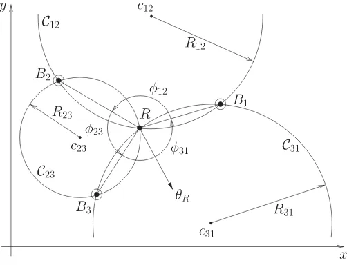
Fig. 3. Triangulation setup in the 2-D plane, using the geometric circle inter-section.Ris the robot.B1,B2, andB3 are the beacons.φi jare the angles
betweenBi,R, andBj.Ci j are the circles that pass throughBi,R, andBj.
Ri jandci jare, respectively, the radii and center coordinates ofCi j.θRis the
robot heading orientation.
All the previous quantities are valid fori=j; otherwise, the circle does not exist. In addition, we have to consider the case φij=kπ,k∈Z. In that case, thesin(.)andcot(.)are equal to
zero, and the circle degenerates as theBiBjline (infinite radius
and center coordinates). In a practical situation, this means that the robot stands on theBiBjline and measures an angleφij=π
when between the two beacons orφij = 0when outside of the
BiBj segment. These special cases are discussed later.
B. Second Part of the Algorithm: Circles Intersection
From the previous section, each bearing angleφij between
beaconsBiandBj constraints the robot to be on a circleCij,
which passes throughBi,Bj, andR(see Fig. 3). The parameters
of the circles are given by (9)–(11). Common methods use two of the three circles to compute the intersections (when they exist), one of which is the robot position and the second being the common beacon of the two circles. This requires to solve a quadratic system and to choose the correct solution for the robot position [18]. Moreover, the choice of the two circles is arbitrary and usually fixed, whereas this choice should depend on the measured angles or beacons and robot relative configuration to have a better numerical behavior.
Hereafter, we propose a novel method to compute this in-tersection by using all of the three circles and by reducing the problem to a linear problem.3To understand this elegant method, we first introduce the notion ofpower center(orradical center) of three circles. Thepower centerof three circles is the unique point of equal power with respect to these circles [13]. The
powerof a pointprelative to a circleCis defined as
PC,p= (x−xc)2+ (y−yc)2−R2 (12)
3The idea of using all the parameters from the three circles is not new and
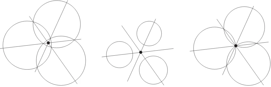
Fig. 4. Black point is the power center of three circles for various configurations. It is the unique point having the same power with respect to the three circles. The power center is the intersection of the three power lines.
where{x, y} are the coordinates ofp,{xc, yc}are the circle
center coordinates, and R is the circle radius. The power of a point is null onto the circle, negative inside the circle, and positive outside the circle. It defines a sort of relative distance of a point from a given circle. Thepower line(orradical axis) of two circles is the locus of points that have the same power with respect to both circles [13]; in other terms, it is also the locus of points at which tangents drawn to both circles have the same length. The power line is perpendicular to the line that joins the circle centers and passes through the circle intersections, when they exist. Monge demonstrated that when considering three circles, the three power lines defined by the three pairs of circles are concurring in the power center [13]. Fig. 4 shows the power center of three circles for various configurations. The power center is always defined, except when at least two of the three circle centers are equal or when the circle centers are collinear (parallel power lines).
The third case of Fig. 4 (right-hand drawing) is particular as it perfectly matches our triangulation problem (see Fig. 3). Indeed, the power center of three concurring circles corresponds to their unique intersection. In our case, we are sure that the circles are concurring since we have
φ31 =φ3−φ1 = (φ3−φ2) + (φ2−φ1) (13)
=−φ23−φ12 (14)
by construction (only two of the three bearing angles are inde-pendent), even in presence of noisy angle measurementsφ1,φ2,
andφ3. It has the advantage that this intersection may be
com-puted by intersecting the power lines, which is a linear problem. The power line of two circles is obtained by equating the power of the points relatively to each circle [given by (12)]. In our problem, the power line ofC12andC23is given by
(x−x12)2+ (y−y12)2−R212 =
where we introduce a new quantitykij which only depends on Cij parameters:
kij=
x2
ij+y2ij−R2ij
2 . (18)
In our triangulation problem, we have to intersect the three power lines, that is to solve this linear system:
⎧
As can be seen, any of these equations may be obtained by adding the two others, which is a way to prove that the three power lines concur in a unique point: the power center. The coordinates of the power center, that is the robot position is given by
which is the signed area between the circle centers multiplied by two. This result shows that the power center exists if the circle centers are not collinear, that is, ifD△= 0. The special case
(D△= 0) is discussed later.
C. First (Naive) Version of the Algorithm
A first, but naive, version of our algorithm consists in applying the previous equations to get the robot position. This method is correct; however, it is possible to further simplify the equations. First, note that the squared radiiR2
ijonly appear in the
expression ofkij[see (18)], we find, after many simplifications,
that
kij =xixj+yiyj+Tij(xjyi−xiyj)
2 (23)
which is much simpler than (11) and (18) (no squared terms anymore). In addition, the1/2factor involved in the circle cen-ters coordinates [see (9) and (10)], as well as in the paramecen-ters kij(18), cancels in the robot position coordinates [see (20) and
(21)]. This factor can thus be omitted. For now, we use these modified circle center coordinates{x′
ij, y′ij}
x′ij = (xi+xj) +Tij(yi−yj) (24)
yij′ = (yi+yj)−Tij(xi−xj) (25)
and modified parameterskij′
k′ij =xixj +yiyj+Tij(xjyi−xiyj). (26)
D. Final Version of the Algorithm
The most important simplification consists in translating the world coordinate frame into one of the beacons, that is solving the problem relatively to one beacon and then add the beacon coordinates to the computed robot position (like Font-Llagunes [18] without the rotation of the frame). In the following, we ar-bitrarily chooseB2 as the origin (B2′ ={0,0}). The other
bea-con coordinates becomeB′
1 ={x1−x2, y1−y2}={x′1, y′1}
and B′
3 ={x3−x2, y3−y2}={x′3, y′3}. Since x′2 = 0 and
y′
2= 0, we havek′12= 0,k′23= 0. In addition, we can
com-pute the value of onecot(.)by referring to the two othercot(.)
because the three angles are linked [see (14)]
T31 = 1−T12T23
T12+T23
. (27)
The final algorithm is given in Algorithm 1.
E. Discussion
The ToTal algorithm is very simple: computations are limited to basic arithmetic operations and only two cot(.). Further-more, the number of conditional statements is reduced, which increases its readability and eases its implementation. Among them, we have to take care of thecot(.)infinite values and the di-vision byD, if equal to zero. If a bearing angleφijbetween two
beacons is equal to0orπ, that is, if the robot stands on theBiBj
line, thencot(φij)is infinite. The corresponding circle
degen-erates to theBiBj line (infinite radius and center coordinates).
The robot is then located at the intersection of the remaining power line and theBiBj line; it can be shown that the
math-ematical limitlimTi j→±∞{xR, yR}exists and corresponds to
this situation.
Like for other algorithms, our algorithm also has to deal with these special cases, but the way to handle them is simple. In prac-tice, we have to avoidInfor NaNvalues in the floating point computations. We propose two ways to manage this situation. The first way consists in limiting thecot(.)value to a minimum or maximum value, corresponding to a small angle that is far be-low the measurement precision. For instance, we limit the value of thecot(.)to±108, which corresponds to an angle of about
±10−8rad; this is indeed far below the existing angular sensor
precisions. With this approximation of the mathematical limit, the algorithm remains unchanged. The second way consists in adapting the algorithm when one bearing angle is equal to0or π. This special case is detailed in Algorithm 2, in which the indexes{i, j, k}have to be replaced by{1,2,3},{3,1,2}, or
{2,3,1}ifφ31 = 0,φ23 = 0, orφ12 = 0, respectively.
The denominatorDis equal to0when the circle centers are collinear or coincide. For noncollinear beacons, this situation occurs when the beacons and the robot are concyclic; they all stand on the same circle, which is called thecritic circumfer-encein [18]. In that case, the three circles are equal as well as their centers, which causesD= 0(the area defined by the three circle centers is equal to zero). For collinear beacons, this is en-countered when the beacons and the robot all stand on this line. For these cases, it is impossible to compute the robot position. This is arestriction common to all three object triangulation, regardless of the algorithm used [14], [18], [31].
The value ofD, computed in the final algorithm, is the signed area delimited by the real circle centers, multiplied by height4.
4Note that the quantityDcomputed in the final algorithm is different from
|D|decreases to0when the robot approaches the critic circle (almost collinear circle center and almost parallel power lines). Therefore, it is quite natural to use|D|as a reliability measure of the computed position. In the next section, we show that1/|D|
is a good approximation of the position error. In practice, this measure can be used as a validation gate after the triangulation algorithm, or when a Kalman filter is used. Finally, it should be noted that the robot orientationθRmay be determined by using
any beaconBi and its corresponding angleφi, once the robot
position is known:
θR =atan2(yi−yR, xi−xR)−φi (28)
where atan2(y, x) denotes the C-like two argument function, defined as the principal value of the argument of the complex number(x+iy).
IV. SIMULATIONS
A. Error Analysis
The problem of triangulation given three angle measurements is an exact calculus of the robot pose, even if these angles are affected by noise. Therefore, the sensitivity of triangula-tion with respect to the input angles is unique and does not depend on the way the problem is solved, nor on the algorithm. This contrasts with multiangulation, which is an overdetermined problem, even with perfect angle measurements. Therefore, we do not elaborate on the error analysis for triangulation, as has been studied in many papers; the same conclusions, as found in [12], [16], [18], [22], [28], and [37], also yield for our al-gorithm. However, in order to validate our algorithm and to discuss the main characteristics of triangulation sensitivity, we
have performed some simulations. The simulation setup com-prises a square shaped area (4×4m2), with three beacons
which form two distinct configurations. The first one is a reg-ular triangle (B1 ={0m,1m}, B2 ={−0.866m,−0.5m},
and B3 ={0.866m,−0.5m}), and the second one is a
line (B1 ={0m,0m}, B2 ={−0.866m,0m}, and B3 =
{0.866m, 0m}). The distance step is 2 cm in each direction. For each point in this grid, we compute the exact anglesφiseen
by the robot (the robot orientation is arbitrarily set to0◦). Then,
we add Gaussian noise to these angles, with zero mean, and with two different standard deviations (σ= 0.01◦,σ= 0.1◦). The
noisy angles are then used as inputs of our algorithm to compute the estimated position. The position error∆dRis the Euclidean
distance between the exact and estimated positions:
∆dR =
(xtrue−xR)2+ (ytrue−yR)2. (29)
The orientation error∆θRis the difference between the exact
and estimated orientations:
∆θR =θtrue−θR. (30)
The experiment is repeated 1000 times for each posi-tion to compute the standard deviaposi-tion of the posiposi-tion error
var{∆dR}and of the orientation error
var{∆θR}. The
standard deviations of the position and orientation errors are drawn in Fig. 5. The beacon locations are represented by black and white dot patterns. The first and second columns provide the result for the first configuration, forσ= 0.01◦, andσ= 0.1◦,
respectively. The third and fourth columns provide the result for the second configuration, forσ= 0.01◦, andσ= 0.1◦,
re-spectively. The first, second, and third rows show the standard deviation of the position error, the standard deviation of the ori-entation error, and the mean error measure1/|D|, respectively. Note that the graphic scales are not linear. We have equalized the image histograms in order to enhance their visual represen-tation and to point out the similarities between the position and orientation error and our new error measure.
Our simulation results are consistent with common three ob-ject triangulation algorithms. In particular, in the first configu-ration, we can easily spot the criticcircumference where errors are large, the error being minimum at the center of this circum-ference. In the second configuration, this critic circumference degenerates as the line passing through the beacons. In addition, one can see that, outside the critic circumference, the error in-creases with the distance to the beacons. It is also interesting to note that1/|D|has a similar shape than the position or orienta-tion errors (except in the particular case of collinear beacons). It can be proven [starting from (20) and (21)] by a detailed sensitiv-ity analysis of the robot position error with respect to angles, that
∆dR ≃
1
|D|∆φ f(.) (31)
Fig. 5. Simulation results giving the position and orientation errors for noisy angle measurements. The beacon positions are represented by black and white dot patterns. The first and second columns provide the results for the first configuration forσ= 0.01◦ andσ= 0.1◦, respectively. The third and fourth columns
provide the results for the second configuration forσ= 0.01◦ andσ= 0.1◦, respectively. Position errors are expressed in meters, the orientation error is expressed in degrees, and the error measure1/|D|is in1/m2. The graphics are displayed by using an histogram equalization to enhance their visual representation and
interpretation.
linearly with angle errors, when they are small (look at the scale of the different graphics). Note that there is a small discrepancy in the symmetry of the simulated orientation error with respect to the expected behavior. This is explained because we usedB1
to compute the orientation [see (28)]. In addition, the histogram equalization emphasizes this small discrepancy.
B. Benchmarks
We have also compared the execution time of our algorithm to 17 other three object triangulation algorithms similar to ours (i.e., which work in the whole plane and for any beacon or-dering). These algorithms have been introduced in Section II,
and have been implemented after the author’s guidelines.5Each algorithm has been running106 times at random locations of
the same square shaped area as that used for the error analysis. The last column of Table I provides the running times on an
Intel(R) Core(TM) i7 920 @ 2.67GHz (6 GB RAM, Ubuntu 11.04, GCC 4.5.2). We used the C clock_gettime function to measure the execution times, in order to yield reliable results under timesharing. It appears that our algorithm is the fastest of all (about 30 % faster than the last best known algorithm of Font-Llagunes [18] and 5 % faster than the recent algorithm of
5The C source code used for the error analysis and benchmarks is available
TABLE I
COMPARISON OFVARIOUSTRIANGULATIONALGORITHMS TO OURTOTALALGORITHM
Ligas [25]). In addition to the computation times, we have also reported the number of basic arithmetic computations, squared roots, and trigonometric functions used for each algorithm. This may help to choose an algorithm for a particular hardware ar-chitecture, which may have a different behavior for basic arith-metic computations, or complex functions such as square root or trigonometric functions. One can see that our algorithm has the minimum number of trigonometric functions, which is clearly related to the times on a classical computer architecture (see Table I). A fast algorithm is an advantage for error simulations, beacon placement, and beacon position optimization algorithms. Note that the algorithm of Ligas also uses the minimum num-ber of trigonometric functions (twocot(.)computations) like ToTal, which explain why both algorithms are basically similar in terms of efficiency. However, the algorithm of Ligas does not provide a reliability measure, contrarily to our algorithm ToTal.
V. CONCLUSIONS
Most of the many triangulation algorithms proposed so far have major limitations. For example, some of them need a par-ticular beacon ordering, have blind spots, or only work within the triangle defined by the three beacons. More reliable meth-ods exist, however they have an increasing complexity or they require to handle certain spatial arrangements separately.
This paper presents a new three object triangulation algorithm based on the elegant notion of power center of three circles. Our new triangulation algorithm, which is called ToTal, natively works in the whole plane (except when the beacons and the robot are concyclic or collinear) and for any beacon ordering. Furthermore, it only uses basic arithmetic computations and two
cot(.)computations. Comprehensive benchmarks show that our
algorithm is faster than comparable algorithms, and simpler in terms of the number of operations. In this paper, we have com-pared the number of basic arithmetic computations, squared root, and trigonometric functions used for 17 known triangula-tion algorithms.
In addition, we have proposed a unique reliability measure of the triangulation result in the whole plane, and established by simulations that1/|D|is a natural and adequate criterion to estimate the error of the positioning. To our knowledge, none of the algorithms of the same family provides such a measure. This error measure can be used to identify the pathological cases (critic circumference) or as a validation gate in Kalman filters based on triangulation.
For all these reasons, ToTal is a fast, flexible, and reliable three object triangulation algorithm. Such an algorithm is an excellent choice for many triangulation issues related to the performance or optimization, such as error simulations, beacon placement, or beacon position optimization algorithms. It can also be used to understand the sensitivity of triangulation with respect to the input angles. A fast and inexpensive algorithm is also an asset to initialize a positioning algorithm that internally relies on a Kalman filter.
APPENDIX
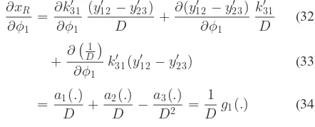
In this section, we detail the sensitivity analysis of the com-puted position. We start by computing the derivative ofxRwith
respect to the first angleφ1
∂xR whereg1(.)is some function of all the other parameters. Similar
results yield for the derivative ofxRwith respect to the second
and third angles,φ2 andφ3, respectively
∂xR
where we assumed that the three infinitesimal increments are equal ∆φ= ∆φ1 = ∆φ2 = ∆φ3. A similar result yields for
the total differential ofyR
∆yR =
1
whereh(.)is some function of all the other parameters. Finally,
wheref(.)is some function of all the other parameters.
REFERENCES
[1] D. Avis and H. Imai, “Locating a robot with angle measurements,”J. Symbol. Comput., vol. 10, pp. 311–326, Aug. 1990.
[2] A. Bais, R. Sablatnig, and J. Gu, “Single landmark based self-localization of mobile robots,” inProc. 3rd Can. Conf. Comput. Robot Vis. (CRV). IEEE Comput. Soc., Jun. 2006.
[3] M. Betke and L. Gurvits, “Mobile robot localization using landmarks,”
IEEE Trans. Robot. Autom., vol. 13, no. 2, pp. 251–263, Apr. 1997. [4] J. Borenstein, H. Everett, and L. Feng, “Where am I? Systems and methods
for mobile robot positioning,” Univ. Michigan, Ann Arbor, MI, USA, Tech. Rep., Mar. 1996.
[5] J. Borenstein, H. Everett, L. Feng, and D. Wehe, “Mobile robot positioning—Sensors and techniques,”J. Robot. Syst., vol. 14, no. 4, pp. 231–249, Apr. 1997.
[6] J. Borenstein and L. Feng, “UMBmark: A benchmark test for measuring odometry errors in mobile robots,” inProc. Soc. Photo-Instrum. Eng., vol. 1001, Philadelphia, PA, USA, Oct. 1995, pp. 113–124.
[7] K. Briechle and U. Hanebeck, “Localization of a mobile robot using relative bearing measurements,”IEEE Trans. Robot. Autom., vol. 20, no. 1, pp. 36–44, Feb. 2004.
[8] M. Brki´c, M. Luki´c, J. Baji´c, B. Daki´c, and M. Vukadinovi´c, “Hardware realization of autonomous robot localization system,” inProc. Int. Conv. Inf. Commun. Technol., Elect. Microelectron., Opatija, Croatia, May 2012, pp. 146–150.
[9] R. Burtch,Three point resection problem, Surveying computations course notes 2005/2006, Ferris State Univ., Big Rapids, MI, USA, 2005, ch. 8, pp. 175–201.
[10] C. Cohen and F. Koss, “A comprehensive study of three object triangula-tion,” inMobile Robots VII. vol. 1831, Boston, MA, USA: SPIE, Nov. 1992, pp. 95–106.
[11] E. Demaine, A. L´opez-Ortiz, J. Munro, Robot localization without depth perception, Proc. Scandinavian Workshop on Algorithm Theory (SWAT), ser. (Lecture Notes Comput. Sci.), vol. 2368. New York, NY, USA: Springer-Verlag, Jul. 2002, pp. 177–194,
[12] A. Easton and S. Cameron, “A gaussian error model for triangulation-based pose estimation using noisy landmarks,” inProc. IEEE Conf. Robot., Autom. Mechatron., Bangkok, Thailand, Jun. 2006, pp. 1–6.
[13] J.-D. Eiden,G´eometrie Analytique Classique. Paris, France: Calvage & Mounet, 2009.
[14] J. Esteves, A. Carvalho, and C. Couto, “Generalized geometric triangula-tion algorithm for mobile robot absolute self-localizatriangula-tion,” inProc. Int. Symp. Ind. Electron., Rio de Janeiro, Brazil, Jun. 2003, vol. 1, pp. 346–351. [15] J. Esteves, A. Carvalho, and C. Couto, “An improved version of the gen-eralized geometric triangulation algorithm,” presented at the Eur.-Latin-Amer. Workshop Eng. Syst., Porto, Portugal, Jul. 2006.
[16] J. Esteves, A. Carvalho, and C. Couto, “Position and orientation errors in mobile robot absolute self-localization using an improved version of the generalized geometric triangulation algorithm,” inProc. IEEE Int. Conf. Ind. Technol., Mumbai, India, Dec. 2006, pp. 830–835.
[17] J. Font-Llagunes and J. Batlle, “Mobile robot localization. Revisiting the triangulation methods,” inProc. IFAC Int. Symp. Robot Control, vol. 8, Santa Cristina Convent, Univ. Bologna, Bologna, Italy, Sep. 2006, pp. 340–345.
[18] J. Font-Llagunes and J. Batlle, “Consistent triangulation for mobile robot localization using discontinuous angular measurements,”Robot. Auton. Syst., vol. 57, no. 9, pp. 931–942, Sep. 2009.
[19] J. Font-Llagunes and J. Batlle, “New method that solves the three-point resection problem using straight lines intersection,”J. Surveying Eng., vol. 135, no. 2, pp. 39–45, May 2009.
[20] H. Hmam, “Mobile platform self-localization,” inProc. Inf., Decis. Con-trol, Adelaide, Australia, Feb. 2007, pp. 242–247.
[21] H. Hu and D. Gu, “Landmark-based navigation of industrial mobile robots,”Int. J. Ind. Robot, vol. 27, no. 6, pp. 458–467, 2000.
[22] A. Kelly, “Precision dilution in triangulation based mobile robot position estimation,”Intell. Auton. Syst., vol. 8, pp. 1046–1053, 2003.
[23] D. Kortenkamp, “Perception for mobile robot navigation: A survey of the state of the art,” Nat. Aero. Space Admin., Tech. Rep. 19960022619, May 1994.
[24] C. Lee, Y. Chang, G. Park, J. Ryu, S.-G. Jeong, S. Park, J. Park, H. Lee, K.-S. Hong, and M. Lee, “Indoor positioning system based on incident angles of infrared emitters,” inProc. Conf. IEEE Ind. Electron. Soc., vol. 3, Busan, Korea, Nov. 2004, pp. 2218–222.
[25] M. Ligas, “Simple solution to the three point resection problem,”J. Sur-veying Eng., vol. 139, no. 3, pp. 120–125, Aug. 2013.
[26] I. Loevsky and I. Shimshoni, “Reliable and efficient landmark-based local-ization for mobile robots,”Robot. Auton. Syst., vol. 58, no. 5, pp. 520–528, May 2010.
[27] M. Luki´c, B. Miodrag, and J. Baji´c, “An autonomous robot localization system based on coded infrared beacons,” inResearch and Education in Robotics (EUROBOT), vol. 161, Prague, Czech Republic, Springer-Verlag, Jun. 2011, pp. 202–209.
[28] C. Madsen and C. Andersen, “Optimal landmark selection for triangulation of robot position,”Robot. Auton. Syst., vol. 23, no. 4, pp. 277–292, Jul. 1998.
[29] C. Madsen, C. Andersen, and J. Sorensen, “A robustness analysis of triangulation-based robot self-positioning,” in Proc. Int. Symp. Intell. Robot. Syst., Stockholm, Sweden, Jul. 1997, pp. 195–204.
[30] C. McGillem and T. Rappaport, “Infra-red location system for navigation of autonomous vehicles,” inProc. IEEE Int. Conf. Robot. Autom., vol. 2, Philadelphia, PA, USA, Apr. 1988, pp. 1236–123.
[31] C. McGillem and T. Rappaport, “A beacon navigation method for au-tonomous vehicles,”IEEE Trans. Veh. Technol., vol. 38, no. 3, pp. 132– 139, Aug. 1989.
[32] V. Pierlot and M. Van Droogenbroeck, “A simple and low cost angle mea-surement system for mobile robot positioning,” inProc. Worksh. Circuits, Syst. Signal Process., Veldhoven, The Netherlands, Nov. 2009, pp. 251– 254.
[33] V. Pierlot, M. Van Droogenbroeck, and M. Urbin-Choffray, A new three object triangulation algorithm based on the power center of three circles, Research and Education in Robotics (EUROBOT), ser. Commun. Com-put. Inf. Sci., vol. 161. New York, NY, USA: Springer-Verlag, 2011, pp. 248–262.
[34] J. Porta and F. Thomas, “Simple solution to the three point resection problem,”J. Surveying Eng., vol. 135, no. 4, pp. 170–172, Nov. 2009. [35] J. Sanchiz, J. Badenas, and F. Pla, “Control system and laser-based sensor
design of an automonous vehicle for industrial environments,”Soc. Photo-Instrum. Eng., vol. 5422, no. 1, pp. 608–615, 2004.
[36] I. Shimshoni, “On mobile robot localization from landmark bearings,”
IEEE Trans. Robot. Autom., vol. 18, no. 6, pp. 971–976, Dec. 2002. [37] S. Shoval and D. Sinriech, “Analysis of landmark configuration for
abso-lute positioning of autonomous vehicles,”J. Manuf. Syst., vol. 20, no. 1, pp. 44–54, 2001.
[38] A. Siadat and S. Vialle, “Robot localization, using p-similar landmarks, optimized triangulation and parallel programming,” presented at the IEEE Int. Symp. Signal Process. Inform. Technol., Marrakesh, Morocco, Dec. 2002.
[39] D. Sinriech and S. Shoval, “Landmark configuration for absolute posi-tioning of autonomous vehicles,”IIE Trans., vol. 32, no. 7, pp. 613–624, Jul. 2000.
[40] H. Sobreira, A. Moreira, and J. Esteves, “Characterization of position and orientation measurement uncertainties in a low-cost mobile platform,” in
Proc. Portuguese Conf. Automat. Contr., Coimbra, Portugal, Sep. 2010, pp. 635–640.
[41] H. Sobreira, A. Moreira, and J. Esteves, “Low cost self-localization system with two beacons,” inProc. Int. Conf. Mobile Robots Competit., Leiria, Portugal, Mar. 2010, pp. 73–77.
[42] O. Tekdas and V. Isler, “Sensor placement algorithms for triangulation based localization,” inProc. IEEE Int. Conf. Robot. Autom., Rome, Italy, Apr. 2007, pp. 4448–4453.
[43] O. Tekdas and V. Isler, “Sensor placement for triangulation-based local-ization,”IEEE Trans. Autom. Sci. Eng., vol. 7, no. 3, pp. 681–685, Jul. 2010.
[45] E. Zalama, S. Dominguez, J. G´omez, and J. Per´an, “A new beacon-based system for the localization of moving objects,” presented at theIEEE Int. Conf. Mechatron. Mach. Vis. Pract., Chiang Mai, Thailand, Sep. 2002. [46] E. Zalama, S. Dominguez, J. G´omez, and J. Per´an, “Microcontroller based
system for 2D localisation,”Mechatronics, vol. 15, no. 9, pp. 1109–1126, Nov. 2005.
[47] O. Fuentes, J. Karlsson, W. Meira, R. Rao, T. Riopka, J. Rosca, R. Sarukkai, M. Van Wie, M. Zaki, T. Becker, R. Frank, B. Miller, and C. M. Brown, “Mobile robotics 1994,” Tech. Rep. 588, Comput. Sci. Dept., Univ. Rochester, Rochester, NY, Jun. 1995 (see http://www.cs.cmu.edu/afs/ cs.cmu.edu/Web/People/motionplanning/papers/sbp_papers/integrated2/ fuentas_mobile_robots.pdf).
[48] T. Heath,Euclid: The Thirteen Books of The Elements. Dover, 1956.
Vincent Pierlot(M’13) was born in Li`ege, Belgium. He received the electrical engineering and Ph.D. de-grees from the University of Li`ege, in 2006 and 2013, respectively.
He is the architect of a new positioning system that has been used during the EUROBOTcontest for sev-eral years. His research interests are mainly focused on electronics, embedded systems, motion analysis, positioning, triangulation, and robotics.
Marc Van Droogenbroeck(M’99) received the elec-trical engineering and Ph.D. degrees from the Univer-sity of Louvain, Louvain-la-Neuve, Belgium, in 1990 and 1994, respectively. While working toward the Ph.D., he spent two years with the Center of Math-ematical Morphology, the School of Mines, Paris, France.