JEJAK
Journal of Economics and Policy
http://journal.unnes.ac.id/nju/index.php/jejak
The Growth Determinant in the Industrial Sector Featured in East
Java Province
Mohtar Rasyid1
1Trunojoyo University, Indonesia
Permalink/DOI: http://dx.doi.org/10.15294/jejak.v8i2.6171
Received: Juli 2015; Accepted: Agustus 2015; Published: September 2015
Abstract
This article aims toanalyzethe main determining factorof growthof industrialsector, especiallythe small scale industriesin East Javaover the past decade. Using theofthe Cobb-Douglas production functionapproach, this research assessedinputfactorconsisting oflabor, capitalandrawmaterials.This study used apooling regression modelto estimate the coefficient of production function fromfourgroups ofselected industries namely:the food industry, textile industry, wood industryandpaperindustry. The results showedthat the sourceof growthfor the industryisstilldominatedbythe physicalgrowth ofinputandnot byproductivity growth. As a result, in the long rungrowth ofthe industry is difficulttobesustainable and relativelyvulnerable toeconomic shocks. Based onthese findingssuggested thatpolicy makersfocus more onefforts toimprove the quality ofinputs, in particularinputqualityhuman resourcesor labor.
Keywords: small scale industries, input driven, productivity driven, sustainable growth
How to Cite: Rasyid, M. (2016). The Growth Determinant in the Industrial Sector Featured in East Java Province. JEJAK: Jurnal Ekonomi Dan Kebijakan, 8(2), 200-214. doi:http://dx.doi.org/10.15294/jejak.v8i2.6171
© 2015 Semarang State University. All rights reserved Corresponding author :
Address: Telang, Bangkalan Stret, Madura, East Java E-mail: [email protected]
INTRODUCTION
Since the 1998 economic crisis, the national economy is quite shocked by the phenomenon known as de-industrialization. One of its indications is the decrease in the utility of industry from time to time (Margono & C, 2004). If the utility of industry in 1996 still reach 82 percent but in 2002 it is dropped to about 63 percent. Based on the number of industries that recorded by the Central Statistics Agency (BPS) nationally in 1996 the number of industry reached 22,997 industries but in 2002 it just remains 21,146 industries. This has an impact to the decrease in production namely in 1996 the percentage of the production index amounted to 120.04, while in 2002 the percentage of the production index becomes around 100.29 (BPS East Java, 2012).
The gloomy portrait of developments in this industry sector was initially triggered by the economic crisis of 1998. However, the economic crisis that lasted nearly a decade ago that certainly can not be considered as a "black sheep" of all kinds of economical root causes. Deeper reviewing to know the structure of the economy is inherently still needs to be more deeply proven (Henstridge, Sourovi, & Jakobsen, 2013). It aims no other than solutions to the problems are satisfactorily obtained and not just rely on the lack-based assumption (Puspita, 2015).
On this basis, this paper will be assessed on the sources of growth on industry sector by taking a sample of small industries in East Java during recent periods. Through this research, it is expected to know the condition of the industrial sector in a comprehensive manner. East Java selected as samples by the reason that this province is one of the largest contributor provinces to the national GDP. Data from the Central Statistics Agency (BPS) shows that
the share of the GDP of East Java in the national production (non-oil) in 2012 reached 16 per cent (Central Bureau of Statistics, 2012). Figures share adrift approximately one percent of Jakarta as the center of the national economy.
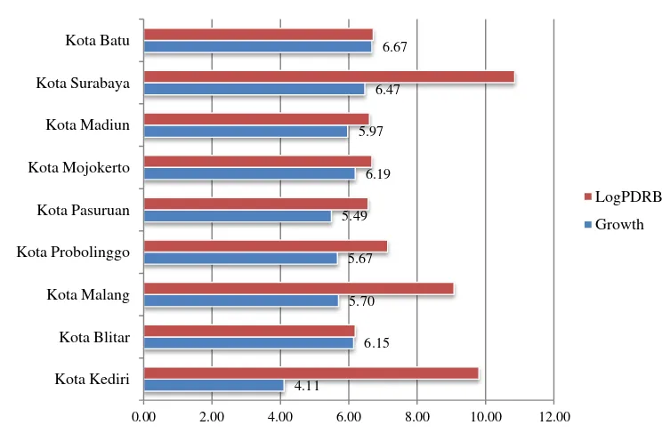
The East Java geographical position which is very strategic puts that region as one of the important economic growth center in Indonesia, especially for eastern region of Indonesia. Some strategic industries located in this region namely: shipbuilding yard (PT. PAL Surabaya), railway industry (PT. INKA Madiun), cigarette factory (Kediri, Kudus and Malang), paper mills (Mojokerto) and cement plants (Gresik). A number of small industries such as leather industry for bags and crafts spread in Sidoarjo even been widely known in the international market (Ministry of Finance, 2012). East Java's growth data for the period of 2000 - 2013 can be seen in Figure 1.
In addition, based on the data found that the development of industrial sector in this province is relatively stable during the study period, thus increasing control over the variables that are not identified and difficult to quantify.
According to Jehle and Reny (2001) production function has a quantitative relationship between output and input. Put simply assumed that the input of capital and labor is the most important input in the production process. The production function shows that output depends on input use and level of technology.
Source: Central Bureau of Statistics, 2000 - 2013
Figure 1.
East Java Growth 2000-2013
The production function is the best approach that can be used to explain why economic growth is different between countries or regions. According to Barro and Martin (2004) the differences that very small at the rate of economic growth will lead to a considerable difference in the standard of living. Further it is stated that, in general, the economic growth in urban areas is relatively faster than non-urban areas (Yuliani, 2015). The city's economy can not grow unless industries in the city use more inputs and adopting better technologies. But this approach can not account for the growth of the city.
Based on the theory of production, output of an industry sector will be affected by the inputs used in the production process. Inputs used in the production process can be grouped into two types, those are the production capital and labor factors input, while the other is technology, efficient production techniques that can be seen through the levels of
productivity. The more input factors used in the production process, the output of the industrial sector will also increasing. Or the output of the industrial sector will be multiplied by the fixed factor input but with a more productive use of inputs that can be done in the presence of better production management or any more efficient production techniques. Thus it can be said that the increase in output of the industrial sector could be caused by the use of more inputs (input driven) or by an increase in productivity (Sari, 2004).
To measure the contribution of each input to output, it can use the standard model of Cobb-Douglas as follows:
ln𝑄𝑖𝑡 = 𝛼 + 𝜑1ln𝑇𝐾𝑖𝑡+ 𝜑2ln𝐾𝑖𝑡 (1) In this case 𝑄 is sectorial additional value; 𝑇𝐾 is the amount of labor used and 𝐾 is a proxy of the purchase of capital goods/ machinery by each industry. The next step is to calculate the
4.11
6.15 5.70 5.67 5.49
6.19 5.97
6.47 6.67
0.00 2.00 4.00 6.00 8.00 10.00 12.00
Kota Kediri Kota Blitar Kota Malang Kota Probolinggo Kota Pasuruan Kota Mojokerto Kota Madiun Kota Surabaya Kota Batu
average contribution of input with the approach of calculation as follows:
𝑞̇ 𝑞 = 𝜑⁄ 1𝑡𝑘̇ 𝑡𝑘⁄ + 𝜑2𝑘̇ 𝑘⁄ + 𝑇𝐹𝑃 (2) Formula above states that output growth is essentially contributed by each input multiplied by the physical growth of each share owned (𝜑1atau𝜑2). If the excess is found in the calculation, then that additional value is contributed by the input productivity or better known as the Total Factor Productivity (TFP).
According to Modjo (2006), TFP is a very important indicator for measuring changes in productivity. These indicators can determine whether or not industrial development strategies implemented can improve productivity. If the industrial sector development strategy can improve the productivity of industrial sector output growth will be a sustained output growth in order to sustain the growth of the output of the bad economic situation. Thus the output growth becomes sustainable growth.
Van der Eng (2006) also says that the high increase in industrial sector output can be caused by two circumstances, namely the use of more inputs (labor, capital, raw materials and fuel); or can also use a fixed input but more productive / efficient. The use of more productive inputs can be carried out in the presence of better production management or any more efficient production techniques. In other words, the source of output growth can be driven by the use of more inputs or by an increase in productivity (productivity driven). Sources of output growth driven by productivity growth indicates that the industrial sector development strategy that is very well implemented.
To trace the path of sectorial growth, sectorial evaluation can also conducted by
using analysis of efficiency. In general, the concept of efficiency can generally be divided into three concepts. First, the technical efficiency, Technical Efficiency basically reflects the ability of certain sectors in order to achieve optimal output level by using certain input level. This efficiency measures production process in generates a certain amount of output by using minimal input. In other words, a production process is said to be technically efficient if the input of an item can no longer be increased without reducing the inputs of other goods.
The second concept is the allocative efficiency. Allocative efficiency reflects the company's ability to optimize the use of its inputs to the pricing structure and technology. Pareto Efficiency terminology is often equated with allocative efficiency to honor the Italian economist Vilfredo Pareto who developed the concept of efficiency inexchange. Pareto Efficiency says that production inputs are used efficiently if the input is no longer possible to be used to increase a business without causing at least one other business situation worse. In other words, if the input is allocated to produce output that is unusable or unwanted by consumer, this means that the input is not used efficiently.
RESEARCH METHODS
The data will be used in this research is secondary data obtained from Indonesia Central Statistics Agency and other agencies associated with this research. In addition, the type of data is data that is combined panel data time series with cross section. The period of data used in this study is from 2003 to 2013, while the type of selected industries is medium and large manufacturing industries which are classified into nine categories.
The variables used in the research model are the output variable, labor variable, capital variable and raw material variable. Output variable is variable depending on which is the output of the manufacturing industry sector in East Java by unit of billion Rupiahs. Input variables are dependent variables that are used as inputs in the industrial sector, where the input variables include the labor force by unit of people, capital by unit of billion Rupiahs, raw materials by unit of billion Rupiahs and fuel by unit of billion Rupiahs.
Furthermore, there are three possible analysis methods or techniques that can be used to estimate coefficients of research model with panel data. According to Wooldridge (2009), the first method is method of ordinary least squares (OLS) while the second and third methods is the fixed effect or random effect, where the two last method is also called the method of generalized least squares (GLS).
In general, the production model (1) can be expressed as follows:
𝑦𝑖𝑡 = 𝜇 + 𝑥𝑖𝑡′ 𝛼 + 𝜃𝑖+ 𝜀𝑖𝑡 (3) Where the error term in the equation (3) is consist of two components. The first component is a specific individual components (= i), which does not change over time. While the second component is the remainder component (= it), which is assumed to be uncorrelated over time.
The use of OLS will be biased and inconsistent when the error terms (i and it) are mutually independent and independent with xjs (for all j and s). There are no autocorrelation in error components structure (i and it) will be indicated by 2 = 0. If there is no autocorrelation in the error components structure then the use of OLS method to estimate the coefficients in production models (2) becomes justified. But if the error terms are correlated over time 2 0, then the use of OLS
method is not justified.
If OLS is not allowed to be implemented in estimating production models (1), the next alternative is by using GLS method. By observing the equation (3), it can determine whether the production model (1) in this study was estimated by OLS or GLS method. If 2 is
equal to zero (2 = 0) then will be equal to
one (=1). This indicates that there is no autocorrelation. Thus, the OLS method can be implemented to estimate the production model (2) in this study. But if is not equal to one ( 1), the GLS method which should be implemented in estimating production models (1).
𝜓 = [ 𝜎𝑠2
𝜎𝑠2+𝑇𝜎𝜃2] (4)
explanatory variables (xit). If there is a correlation between the individual effects (i) and explanatory variables (xit) then the use the random effects estimator will result in inconsistent estimation. However, if there is a correlation between the individual effects (i) and explanatory variables (xit) then it can be overcome by using fixed effects estimator model. This fixed effects model can eliminate the influence of individual effects (i) in the production model (3).
Therefore, if there are two kinds of tests that can be used to determine whether the production model (3) in this study will be estimated by OLS or GLS method which includes fixed effects or random effects. The first test is by using Breusch-Pagan test (BP test) this test is used to confirm whether the production model (3) estimated by using OLS or GLS. BP null hypothesis of the test is the 2 = 0, which
means no autocorrelation, while the alternative hypothesis is 2 0, which means there is
autocorrelation. If the null hypothesis is accepted then the production models (3) estimated by using the OLS method, but if the null hypothesis is rejected then the production model (3) estimated by GLS method.
If the GLS method chosen to estimate the production model (3) then the next step is to perform Hausman test. This test is used to determine whether the production model (3) using fixed effects or random effects. The null hypothesis of the Hausman test is no
correlation between individual
effects (i) and explanatory variables (xit) in the production model (3). This indicates there is no significant difference between the individual effects (i) and explanatory variables (xit). Thus using random effects will be consistent and efficient. While the alternative hypothesis of Hausman test is individual effects (i) and explanatory variables (xit) are correlated. So there is significant difference between
the individual effects (i) and explanatory variables (xit). Thus using fixed effects estimator will be consistent. Therefore, in general, one can say if it is not reject the null hypothesis so random effect method will be used, otherwise it rejects the null hypothesis, the method of fixed effects that will be used.
To measure the technical efficiency, in Charnes, and Chooper (BCC) model, which was introduced in 1984. CCR model is the model most often used in DEA models. The following will be describe these two models:
1. Constant Return to Scale (CRS)
The model was developed by Charnes, Cooper and Rhodes (CCR Model) in 1978. DEA Model by CRS design assumes that the production process following the CRS, which means that, any proportionally increase of input in certain percentage will increase the output by the same percentage. This assumption is only valid if every business unit observed has been producing at full capacity (optimum scale). Efficiency with this CRS assumption will produce overall technical efficiency. To get the overall efficiency score for the company i(θ), which has one input x and one output y, is obtained by solving a system of linear equations as follows:
n = number of business units observed x 1 = input x of business unit 1
λ = vector of the constant
2. Variable Return to Scale (VRS)
The second model was developed by Banker, Charnes, and Cooper (BCC Model) in 1984 and is a development model of the previous model, the CCR. In real conditions, often competition and financial constraints can lead to a business unit not operating at optimal scale. Though, the CRS assumption is true if the business unit observed were operating at optimal scale. With this purpose Banker, Charnes and Cooper (1984) introduced a VRS DEA model. Technical Efficiency (TE) calculated using VRS models are referred to as Pure Technical Efficiency, hereinafter referred to as technical efficiency. By doing frontier estimation by using CRS and VRS models, it can be conducted decomposition of Overall Technical Efficiency into Pure Technical Efficiency and Scale Efficiency. Then the mathematical calculation is as follows:
OTE = PTE x SE
DEA model which is based on input with VRS assumption can be shown by linear
n = number of business units observed x1 = input x of business unit 1
y1 = output y of business unit 1
In this case N1 'λ = 1 is convexity constraint, N1 is the vector N x 1and θ is a scalar
quantity (1 ≥ θ ≤ ∞). For a number of N DMU,
with input amounted of A and output of B on each DMU, yi is the output vector B xN and xi is
the input vector AxN. Y and X consists of data for the entire DMU. If linear programming problem is without convexity constraint (N1'λ = 1), then it became a DEA model based on input of CRS assumption.
This research is using panel data that allows in calculating the change in productivity as well as outlines in the form of changes in technology and changes in technical efficiency. DEA method used was malmquist orientation index of input and VRS assumption. The value which is greater than one indicates that there is a positive growth of Total Factor Productivity (TFP) from period t to period t + 1. This index is the geometric mean of the two output-based Malmquist TFP indices. One of the index used technology in period t and the other used the technology in period t + 1. Malmquist index value that is less than one, then the value indicates that the UKE experienced a decline in total productivity.
RESULTS AND DISCUSSION
Based on the analytical techniques described above it can be concluded that the use of fixed effect method is more precise than the methods of random effect. More completely, the results of calculations can be illustrated by the print-out Eviews in Table 1.
industries in East Java during the past decade working in conditions of increasing return to scale.
Partially, it can be explained by assuming that the other variables constant, the increase in total employment by 1% on average would increase output by 0.764%. Increasing the amount of capital by 1%, assuming other variables Constance, will result in an increase in output by 0.097%. Furthermore, assuming the same, that all other variables held constant, an
increase in the quantity of raw materials amounting to 1%, then the average will increase the output of the industrial sector amounted to approximately 0.83%. The next stage after calculating the regression coefficients for each input factor being tested is to calculate the productivity of each input. The following analysis summarizes the growth in output over the study period (2003-2013), the growth of the amount of labor, capital growth as well as raw materials during the same period.
Table 1.
Estimated Production Function Model of Cobb-Douglas
Variable Coefficient Std. Error t-Statistic Prob.
LOG(LABOR?) 0.764835 0.121211 6.309964 0.0000
LOG(KAPITAL?) 0.097722 0.028218 3.463117 0.0014
LOG(RAW?) 0.834478 0.065493 12.74149 0.0000
Fixed Effects
31--C -6.725270
32--C -6.399949
33--C -6.019189
34--C -5.528658
R-squared 0.971923 Mean dependent var 22.71281 Adjusted R-squared 0.967370 S.D. dependent var 1.113791 S.E. of regression 0.201192 Sum squared resid 1.497701
Log likelihood 11.93239 F-statistic 213.4680
Durbin-Watson stat 1.607882 Prob(F-statistic) 0.000000 Source: Data processed
Table 2.
Growth of Output, Input and Productivity
ISIC Growth
Output
Growth Labor
Growth Capital
Growth
Raw Productivity
31 0.208159 0.0197129 3.9137781 0.202046 -0.35798
32 0.793453 0.1763591 10.6670401 0.202604 -0.55290 33 0.187792 -0.0479145 0.8897521 0.178015 -0.01106
34 0.334611 0.0412821 0.4955848 0.337059 -0.02666
Some things that can be interpreted according to Table 2 above is that it is basically a small industrial sector output growth in East Java during the study period is basically an average relatively high, reaching approximately 30%. The growth experienced by sub-sectors of the textile industry (ISIC 32).
However, as also noted in the table above is that despite growing relatively well but the absorption of labor is still quite low. On the average absorption of labor is equal to an average of 4% with the lowest absorption is in the timber industry sub-sector (ISIC 33). Absorption of labor for the sector in question actually decline (-4.7%).
Further, the growth which uses the relatively high capital is owned by the textile industry. Furthermore, the food industry (ISIC code 31) also increased relatively high in the use of capital. Development of the use of capital during the study period was the lowest in the sub sectors of the paper industry (ISIC 34).
When compared with the three other input factors, the use of inputs such as raw materials has developed nearly equal to the four sub-sectors studied. On the average development of the use of raw materials reached almost 23% per year with details of sub-sectors of food and textile industry grew by 20% per year; timber industry sub-sector by 17% and paper industry sub-sector achieved an average 33% per year.
Among some of the interesting fact to note is that the productivity of inputs for each sub-sector studied is having a negative coefficient. These results can be interpreted that the sources of growth in small industrial sector in East Java today is still input driven compared to the productivity driven.
As previously mentioned, input driven-based growth in many cases are relatively
unstable and can not guarantee the achievement of sustainable growth. Another fact that also can not be forgotten is that such sources of growth are more dependent on capital and raw materials and not in the labor supply.
This fact may explain why the national industry is very sensitive to changes in exchange rates for a given percentage of imports of capital goods and raw materials as long as this is still dominant. Ironically, each of turmoil (shock) in the industrial sector is more often followed by massive layoffs event. With labor productivity is relatively low then the possibility of "repatriation" of labor often is considered as the only logical completion of crisis.
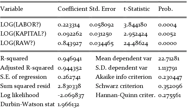
To test the resilience of the model (robustness check), then the main regression analysis model will be evaluated with an alternative model, the model of pooling and random effects models. As a first step, the model estimation is conducted by using a pooling approach. More estimation results can be noticed in Table 3.
Table 3.
Estimation Model
Pooled Least Square
Variable Coefficient Std. Error t-Statistic Prob.
LOG(LABOR?) 0.223314 0.058092 3.844180 0.0004 LOG(KAPITAL?) 0.092262 0.031250 2.952424 0.0052 LOG(RAW?) 0.843927 0.034465 24.48624 0.0000
R-squared 0.946941 Mean dependent var 22.71281 Adjusted R-squared 0.944352 S.D. dependent var 1.113791 S.E. of regression 0.262741 Akaike info criterion 0.230447 Sum squared resid 2.830338 Schwarz criterion 0.352096 Log likelihood -2.069837 Hannan-Quinn criter. 0.275561 Durbin-Watson stat 1.966132
Source: Data processed
Redundant test results can be referred to briefly consider in the summary of Table 4 as follows:
Table 4.
Redundant Fixed Effect Test
Redundant Fixed Effects Tests Pool: Untitled
Test cross-section fixed effects
Effects Test Statistic d.f. Prob.
Cross-section F 9.366905 (3,37) 0.0001
Cross-section Chi-square 24.860774 3 0.0000
Source: Data processed
Table 4 above displays the results of the data redundant fixed effect processing. The test is conducted by evaluating the significance of the cross section in the data unit. If the characteristics of the respective sub-sectors of the industry have differences with each other, then the cross-section coefficient would be significant. Conversely, if the unit sub-industries analyzed are relatively homogeneous, then the cross-section unit tested should not be significant. In this case, the analysis should be conducted by using the
With degrees of freedom, each for 3 and 37, the statistical probability of F recorded at 0.0001. This value is certainly very far from the conventional cut-off value of 0.05. In other words, the presence of dummy cross-section in the model is very significant.
Similar conclusions can also be seen by Chi-square statistics. The calculations show that the Chi-square statistic of 24.86 was also very significant. These results reaffirm that turns the unit cross-section is very significant. Thus, the difference between the units of the sub-sector in this case is very significant.
Based on the results of these discussions it is clear it can be concluded that between the Pooled Least Square approach versus Fixed Effect approach, the last one is more superior (Fixed Effect). Abandonment to different
elements of this cross-section will potentially produce biased estimator.
Results of previous discussion clearly assert that the estimation of Fixed Effect Model is more superior than the Pooled Least Square Model. The next step to determine the best model is by comparing performance of Fixed Effect Model with other alternative models, Random Effect Model. The principal idea of random models is the specific elements of each sub-sector can be included as an element in a disturbance or error term.
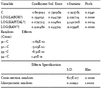
Thus, it is necessary to estimate the adjustment such that the estimator obtained will be efficient. The estimation results of random effect can be observed in Table 5. By significance, estimators obtained are all significant in the conventional level (5%).
Table 5.
Estimation of
Random Effects
Model
Variable Coefficient Std. Error t-Statistic Prob.
C -1.605092 0.730989 -2.195781 0.0340
LOG(LABOR?) 0.234032 0.044750 5.229724 0.0000 LOG(KAPITAL?) 0.079725 0.024601 3.240708 0.0024 LOG(RAW?) 0.920460 0.043719 21.05396 0.0000 Random Effects
(Cross)
31--C -2.69E-12
32--C -5.03E-12
33--C -6.32E-12
34--C 1.40E-11
Effects Specification
S.D. Rho
Cross-section random 6.17E-07 0.0000
Idiosyncratic random 0.201192 1.0000
However, the magnitude of regression coefficients obtained is relatively different from the results of previous estimation. Specific element of each cross-section in theory can be put into two distinct elements: the intercept element or disturbance element. If in the intercept elements, then this element explicitly represents all the variables outside the model that affect the dependent variable. If the element outside the model has a correlation with the variables included in the model, the estimated regression coefficients of variables in the model will be rectified. Yet, this correction coefficient will still produce an unbiased estimator.
Conversely, if the specific elements of the cross-section entered as a random element, then the potential for bias due to the effects of the elements outside the model can not be isolated. That is, if an element outside the model has the effect of a strong correlation with the variables in the model, then putting a
specific element of a cross-section into an element of random will not solve the problem of bias.
Theoretically, the model of fixed effect is relatively more consistent because it can overcome the problem of bias. The random effect model is more precisely relates to efficiency estimator. If both of these approaches give approximately the same estimator, then random effect approach is certainly preferable. Conversely, if the estimator of fixed effect and random effect is very different then the estimator of fixed effect will give more consistent results.
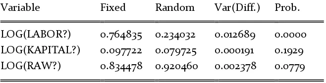
To determine appropriate estimation method, can be tested by Hausman test. In methodology, this test is used to evaluate differences regression coefficient generated by Model Fixed Effects versus Model Random Effect. The results of its calculation can be noted in the following table:
Table 6.
Hausman Test: Fixed versus Random
Test Summary
Chi-Sq.
Statistic Chi-Sq. d.f. Prob.
Cross-section random 28.100714 3 0.0000
Cross-section random effects test comparisons:
Variable Fixed Random Var(Diff.) Prob.
LOG(LABOR?) 0.764835 0.234032 0.012689 0.0000 LOG(KAPITAL?) 0.097722 0.079725 0.000191 0.1929 LOG(RAW?) 0.834478 0.920460 0.002378 0.0779
Table 6 above shows the results of Hausman test to compare the results of the Fixed Effect estimation with Random Effect estimation. In general, the results show that the difference between the two estimators is significantly differing. Chi-square value of this test is 28.1 and highly significant even though in 1% level testing.
To see the magnitude of the difference between the two coefficients above, can be noticed in the panel below of Table 6. It can clearly be seen that the coefficient of labor (Labor) of fixed effect estimation result is amounted to 0.764 and the random effect estimation is amounted to 0.234. Thus there is coefficient difference of 0.012689. The difference was statistically highly significant. Furthermore, the coefficient of capital for fixed effect amounted to 0.097 and the random effect of 0.079. There are differences in the amount (magnitude), although the difference is statistically not significant.
Furthermore, the regression coefficients for the variables of raw materials (raw) generated by the estimator of fixed effect amounted to 0.834 and the random effect of 0.920. The coefficient difference is significant in significance level of 5% on the one end.
Based on the discussion about consistent estimator, it can be produced some important results. First, there is evidence that the variation between the cross section units in this study is differ significantly. Thus, the use of a homogeneous model of inter-unit sub-sector is becoming less valid. In this case the pooling regression model relatively inferior compared to other estimators.
Second, the specific differences between the sub-sectors units analyzed in further tests proved to be more suitable assumed as part of
the intercept compared with random elements. Based on these findings, it can be ascertained that the fixed effect model is more superior than the other estimation model. Thus, the fixed effect estimator as presented in Table 1 is relatively more appropriate than other alternative estimation model.
In accordance with the discussion of the regression model analysis of the estimated resources of featured industrial sector growth, as presented in Table 2 have the strong support methodology. Thus, the conclusions about the driven input phenomenon in the featured industrial sector, research questions that also will be answered is related to the growth path that can be performed by each sector so that the growth is more optimal. For that it is necessary to the calculation of technical efficiency in all sub-sectors to determine which sectors have the most efficient performance.
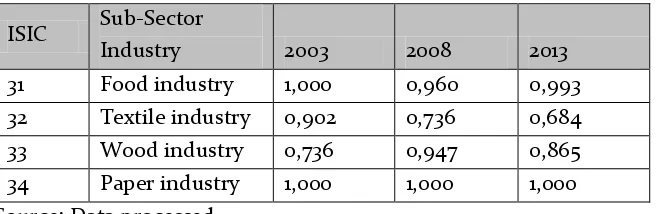
Table 7. Calculation of Technical Efficiency, 2003, 2008 and 2013
ISIC Sub-Sector
Industry 2003 2008 2013
31 Food industry 1,000 0,960 0,993
32 Textile industry 0,902 0,736 0,684
33 Wood industry 0,736 0,947 0,865
34 Paper industry 1,000 1,000 1,000
Source: Data processed
If conducted any addition of the unit of analysis, the final result and conclusions obtained will also be different. To calculate the technical efficiency of featured industrial sub-sectors in East Java, this study will assess efficiency in some period of time. It is intended to test the consistency of calculation results over time. The result of technical efficiency calculation can be considered in table 7.
The result of the calculation of technical efficiency sub-sector industry in East Java can be noted in Table 7 above. Based on the above findings can be seen that during the study period, the paper industry (ISIC code 34) consistently had the highest level of efficiency compared with three other industry groups.
Some industries have a high degree of efficiency changes. The food industry has a level of efficiency that is relatively consistent despite several periods with minor changes. The textile industry in fact has an efficiency level relative decline from year to year compared to other industries. In 2003, the efficiency of this industry reached almost 100% (90.2% to be exact). Over time, the textile industry experienced a decrease in efficiency. In 2008 the level of efficiency achieved amounted to 73.6% and decreased to 68.4% in 2013. Furthermore, the timber industry was recorded as an industry with the unstable level of efficiency. In 2003 the level of technical efficiency achieved in the industry amounted to 73.6%. The efficiency of the timber industry in 2008 increased to
94.7%. But in 2013 the efficiency achieved by this industry was 86.5%. Based on these results it is clear that the featured industry which has the highest efficiency in East Java is the paper industry. Therefore, to improve the overall industry performance, the development of featured industry can follow the growth path of the paper industry. One of the featured industries with a relatively high degree of efficiency is the food industry.
CONCLUSION
The calculations show that the source of growth in the industrial sector in East Java during the study period was more contributed by the elements from the additional of input (input driven). The structure of sectoral growth as it is believed to be unable to generate sustainable economic growth. The structure of stable economic growth should have been more dominated by growth derived from the growth of productivity.
quality of human or more specifically the quality of labor, in addition will improve the welfare for the workers themselves, but also believed to ensure the achievement of sustained economic growth and relatively strong in responding to economic shocks both from within and from outside.
Some industries may be used as a raw model of the development of featured industry in East Java. One of the sub-sectors in question is the paper industry. As one of the centers of the paper industry in Indonesia, East Java can be used as a model of the development of the paper industry in the country. Conversely, the textiles industry, which have relatively decreases efficiency from year to year is an industry that should receive special attention from policy makers. Given the potential of the textile industry with the potential for domestic and export markets are still very wide, very unfortunate if the textile industry has the performance (efficiency), which continues to decline. In harmony with the findings in this study, improving the quality of human resources combined with more efficient use of resources will produce a steady and sustainable growth rate.
REFERENCES
Badan Pusat Statistik. (2012). Perkembangan Beberapa Indikator Utama Sosial Ekonomi Indonesia 2012.
Jakarta: Badan Pusat Statistik.
Barro, R. J., & Sala-i-Martin, X. (2004). Economic Growth: Second Edition. London: MIT Press.
BPS Jawa Timur. (2012). Jawa Timur Dalam Angka.
Surabaya: Badan Pusat Statistik.
Henstridge, M., Sourovi, & Jakobsen, M. (2013). Growth in Indonesia: Is it Sustainable? Drivers of Economic Growth. Oxford Policy Management. Ismail, R., Sulaiman, N., & Jajri, I. (2014). Total Factor
Productivity and Its Contributions to Malayasia's Economy Growth. Research Journal of Applied Sciences, Engineering and Technology , 4999-5005.
Jehle, G. A., & Reny, P. J. (2001). Advanced Microeconomic Theory: Second Edition. New York: Addison Wesley.
Kementrian Keuangan RI. (2012). Tinjauan Ekonomi dan Keuangan Daerah. Jakarta: Kementrian Kuangan RI.
Margono, H., & C, S. S. (2004). Efficiency and Productivity Analyses of Indonesian Manufacturing Industries. Southern Illinois University Carbondale.
Modjo, M. I. (2006). Total Factor Productivity in Indonesian Manufacturing: A Stochastic Frontier Approach. Monash University.
Puspita, D. W. (2015). Analisis Determinan Kemiskinan di Provinsi Jawa Tengah. JEJAK Journal of Economics and Policy, 8 (1).
Sari, D. W. (2004). The Source of Growth of Indonesia's Manufacturing Industry. The 29th FAEA Annual Conference (pp. 1-19). Kuala Lumpur: Institute Integrity of Malaysia.
Van der Eng, P. (2006). Accounting for Indonesia's Economic Growth: Recent Past and Near Future.
Brisbane: University of Queensland.
Wooldridge, J. M. (2009). Introductory Econometrics, A Modern Approch . Cengage Learning.