Capital Budgeting versus Market Timing:
An Evaluation Using Demographics
STEFANO DELLAVIGNA and JOSHUA M. POLLET∗
ABSTRACT
Using demand shifts induced by demographics, we evaluate capital budgeting and market timing. Capital budgeting implies that industries anticipating positive de-mand shifts in the near future should issue more equity to finance greater capacity. To the extent that demand shifts in the distant future are not incorporated into eq-uity prices, market timing implies that industries anticipating positive shifts in the distant future should issue less equity due to undervaluation. The evidence supports both theories: new listings and equity issuance respond positively to demand shifts during the next 5 years and negatively to demand shifts further in the future.
THE DETERMINANTS OF EQUITYissuance are the subject of an ongoing debate in
corporate finance. Are initial public offerings (IPOs) and seasoned offerings best explained by the demands for external finance, or are they driven by market timing in response to company misvaluation?
Capital budgeting holds that firms issue equity (and debt) to invest the pro-ceeds in positive net present value (NPV) projects, for example, to expand production when demand is high (Modigliani and Miller (1958)). Market tim-ing instead holds that firms issue equity to take advantage of misprictim-ing by investors (Stein (1996),Baker, Ruback, and Wurgler (2007)).
One crucial difficulty in evaluating these theories is the lack of exogenous proxies for investment opportunities, on the one hand, and for misvaluation, on the other hand. For instance, the relationship between the market-to-book ratio and corporate decisions could reflect investment opportunities (Campello
and Graham (2012)), mispricing related to accruals or dispersion of opinion
(Gilchrist, Himmelberg, and Huberman (2005),Polk and Sapienza (2009)), or
both (Hertzel and Li (2010)). These issues are also linked to whether market-to-book is a proxy for risk (Fama and French (1992)) or a measure of mispricing relative to accounting fundamentals (Lakonishok, Shleifer, and Vishny (1994)).
∗DellaVigna is from the Department of Economics, University of California, Berkeley. Pol-let is from the Department of Finance, University of Illinois at Urbana-Champaign. We thank Malcolm Baker; Patrick Bolton; James Choi; Kenneth French; Ron Giammarino; Gur Huberman; Christopher Polk; Michael Weisbach; Jeffrey Wurgler; and audiences at Amsterdam University, Columbia University, Dartmouth College, Emory University, Harvard University, Rotterdam Uni-versity, Tilburg UniUni-versity, UCLA, University of Illinois at Urbana-Champaign, the 2008 AFA Annual Meetings, and the 2008 Texas Finance Festival for comments. We also thank Jay Ritter for providing IPO data. Finally, we gratefully acknowledge the support of the NSF through grant SES-0418206.
We use demographic variables as proxies for both in a novel evaluation of these two theories. We consider industries that are affected by predictable shifts in cohort sizes, such as breweries and long-term care facilities. These industries have distinctive age profiles of consumption. Therefore, forecastable changes in the age distribution produce forecastable shifts in demand for var-ious goods. Even though these demand shifts only capture a small component of the variation in investment opportunities and mispricing, they are exoge-nous from the perspective of the manager. As such, they allow us to address the endogeneity problem and identify separately the managerial response to variation in investment opportunities and mispricing.
We distinguish between shifts that will affect an industry in the near future, up to 5 years ahead, and shifts that will occur in the more distant future, 5 to 10 years ahead. As the model inSection Idemonstrates, traditional capital budgeting indicates that industries affected by positive demand shifts in the near future should raise capital to increase production. Positive demand shifts increase marginal productivity and the optimal level of investment; in turn, the desire for more investment induces demand for additional capital. Therefore, demand shifts due to demographics in the near future should be positively related to equity issuance.
Another prediction relies on the assumption that investors are short-sighted and hence partially neglect forecastable demographic shifts further in the future (5 to 10 years ahead). Indeed, demand shifts due to demographics 5 to 10 years ahead significantly predict industry-level abnormal returns
(DellaVigna and Pollet (2007)). In our model, we assume that managers in
a particular industry have longer foresight horizons than investors—perhaps because managers usually develop in-depth knowledge essential to long-term planning. Under this assumption, demand shifts in the distant future serve as proxies for mispricing and managers react to this mispricing by modifying their equity issuance decisions. Companies in industries with positive demand shifts 5 to 10 years ahead will tend to be undervalued and managers respond by reducing equity issuance (or repurchasing equity). Conversely, companies in industries with negative demand shifts 5 to 10 years ahead will tend to be overvalued, and managers react by issuing additional equity. This analysis as-sumes that the announcement of issuing or repurchasing equity does not cause investors to fully eliminate the mispricing.
We also consider a case in which time-to-build considerations create a trade-off between raising equity to finance investment and repurchasing equity to exploit mispricing. A company facing high demand growth due to demographics 5 to 10 years ahead would like to repurchase shares (market timing) but also invest (capital budgeting). Unlike in the standard case, time-to-build induces a trade-off between the two because the company cannot postpone investment to the later period. Hence, the above predictions are attenuated in high time-to-build industries compared to low time-time-to-build industries.
issuing equity. Market timing does not provide a clear prediction about the relation between long-term demand shifts and debt issuance.1
To summarize, capital budgeting predicts that demand shifts due to demo-graphics in the near future should be positively related to debt and equity is-suance, while market timing suggests that demand shifts further in the future should be negatively related to equity issuance. We note that the two predic-tions are not mutually exclusive. InSection II, we describe the construction of demand shifts due to demographics (obtained combining cohort size forecasts and estimates of age profiles of consumption) and introduce the measures of external financing.
In Section III, we analyze the impact of demographics on the likelihood of
IPOs and on additional equity issuance by listed firms in an industry. We find that demand shifts due to demographics up to 5 years ahead are positively related to the ratio of new listings to existing listings, consistent with capital budgeting. Demand shifts due to demographics 5 to 10 years ahead are sig-nificantly negatively related with this IPO measure, consistent with market timing. We find similar results for the ratio of listing with large additional equity issuance to existing listings, our measure of secondary equity issuance. As predicted, these results are stronger for less competitive industries and for industries with lower time-to-build.
We also consider the impact of demand shifts on debt issues and repurchases. The evidence regarding debt is imprecisely estimated. For most of the speci-fications, the sign of the coefficient estimates for demand shifts in the near future is consistent with capital budgeting but the estimates are not statisti-cally significant. There is also little statistical evidence that demand shifts in the distant future are related to debt policy.2
Finally, we provide evidence on the channels underlying these results. The model in Section II links equity and debt decisions to demographic shifts through investment. Indeed, we show that positive demand shifts up to 5 years ahead increase investment as well as research and development (R&D). These results provide evidence that investment, broadly defined, is a determinant of the demand for external capital.
In Section IV, we discuss five alternative explanations: signaling, agency
problems, large fixed costs of equity issuance, globalization, and unobserved time patterns. We find that these potential alternatives are not likely to gen-erate our findings.
This paper is related to the substantial empirical literature about mar-ket timing.3 Relative to this literature, we consider a novel exogenous proxy
1The extent to which debt is mispriced when equity is mispriced is unclear. Debt issuance may
be a substitute for equity issuance if debt is less mispriced than equity.
2However, in a few specifications long-term demand shifts are negatively related to debt
repur-chases. This result could support market timing if debt is used as a substitute for equity, that is, if undervalued firms repurchase equity but do not repurchase debt due to financing constraints.
3SeeBaker, Ruback, and Wurgler (2007),Campello and Graham (2012),Carlson, Fisher, and
for mispricing. The paper is also related to the literature on corporate re-sponse to anticipated demand shifts (Acemoglu and Linn (2004),Goolsbee and
Syverson (2008),Ellison and Ellison (2011)). Unlike these papers, we focus on
equity and debt financing decisions. This paper is also associated with the evi-dence on the effect of demographics on corporate outcomes and aggregate stock returns (Poterba (2001), Acemoglu and Linn (2004)). Finally, we extend the discussion regarding the role of attention allocation in economics and finance.4
Our evidence suggests that the inattention of investors with respect to long-term information (DellaVigna and Pollet (2007)) affects corporate financing decisions.
I. A Model
We consider a simple two-period model of investment and equity issuance. The investment opportunity is a long-term project that can be financed in ei-ther period 1 or 2; the cash flow from this project is realized at the end of period 2. In the second period, the manager and investors have the same (correct) expectations about the expected value of the investment opportunity. However, in the first period investors do not correctly foresee the expected value of the investment opportunity in period 2, since the level of demand is beyond their foresight horizon.5 Only the manager correctly foresees the expected value of
the investment opportunity since he has a longer foresight horizon. Therefore, limited attention induces time-varying asymmetric information between in-vestors and the manager. We also consider the rational expectations case in which investors have correct expectations throughout.
To match the empirical evidence, it helps to think of the two periods as approximately 5 years apart. We assume that investors are naive about their limited foresight, and hence, do not use the equity issuance policy to make inferences about the information known by the manager. Also, since our goal is to focus on the impact of investor foresight, we do not consider other forms of asymmetric information. We assume that the manager maximizes the price per share for existing shareholders that hold their shares until the end of period 2. We capture time-to-build aspects associated with production by considering two polar cases: (i) investment in period 1 or 2 is equally productive (no time-to-build), and (ii) investment in period 2 is completely unproductive (severe time-to-build). The second case describes industries in which cost-effective in-vestment in new plants must begin many years before production, that is, in period 1 and not in period 2. For example, it is much less costly to build a new aircraft assembly plant over a multiyear period than building it in 1 year.
The firm chooses the level of investments, I1 and I2∈[0,∞), with a
gross product αf(I1+ g(I2)) in period 2, where g(.) captures the (potential)
4SeeBarber and Odean (2008),Cohen and Frazzini (2008), Daniel, Hirshleifer, and
Subrah-manyam (1998),DellaVigna and Pollet (2009),Hirshleifer, Lim, and Teoh (2009),Hong and Stein (1999),Huberman and Regev (2001), andPeng and Xiong (2006).
5This mistake in expectations is an error in the perception of the average return for the project.
time-to-build considerations. The marginal productivity of investment in the project is determined byα= {α, α}. When demand due to demographics is high,
αis high:α=α; when demand due to demographics is low,αis low:α=α < α. We assume that the production function is increasing and concave: f′(I)>0
and f′′(I)<0 for all I≥0. To guarantee positive and finite investment for
each project, we assume standard limiting conditions: limI→0 f′(I)= ∞ and
limI→∞ f′(I)=0.For convenience, we consider two limiting cases for g(I). In
the absence of time-to-build, g(I)=I, that is, there does not exist a cost of delaying the investment until period 2. In the presence of substantial time-to-build,g(I)=0,that is, there exists a prohibitive cost of delaying investment to period 2.
The manager uses internal funds or raises external finance (equity) in pe-riod 1 or 2 to undertake investments I1 and I2. Equity is the only financial
instrument that is affected by the limited foresight horizon of the investor. (We discuss an extension with riskless debt at the end of this section.) In period 1, the firm has cashC available and Nshares outstanding. We assume that the financing constraints are only binding when demand is high. The firm always has enough cash to undertake the first-best investment with low demand α, but not enough cash to undertake the first-best investment with high demand
αwithout some equity issuance.
The firm can issuen1shares in period 1 (at price P1) andn2shares in period
2 (at price P2). Equity issuance in either period can be negative, that is, we
allow the firm to repurchase equity. We assume that there is a maximum amount of total equity issuance or repurchases: 0<N≤N+n1+n2≤Nand
N≤ N+n1≤ N, with N<N. These technical assumptions rule out infinite
share issuance and complete share repurchase. We let Nbe large enough that it is always possible to issue sufficient equity to finance the first-best levels of investment, but it may not be optimal for the manager to do so. Finally, to break ties when the firm is indifferent with respect to equity issuance, we assume that the manager incurs an extremely small fixed cost K each time equity is issued or repurchased.
The manager maximizes the price per share for the long-term shareholders, that is, total firm value scaled by the number of shares outstanding at the end of period 2. The firm’s value is the sum of the initial cash holdingsC, the total equity raised,n1P1+n2P2, plus the value of the investment,αf(I1+g(I2)), net
of the investment expense, I1+I2. The interest rate between the two periods
is normalized to zero. The manager’s maximization problem is
max
n1,n2,I1,I2 1 N+n1+n2
(C+n1P1+n2P2+αf(I1+g(I2))−I1−I2), (1)
subject to
I1≤C+n1P1,
I1+I2≤C+n1P1+n2P2,
N≤ N+n1+n2≤ N,
Although the manager knows the realization of the demand parameterα, in-vestors in period 1 neglect demographic factors and make a forecastα, with
α≤α≤α. This assumption captures the (potential) short-sightedness of in-vestors. In period 2, investors and managers instead agree about the level of demand, since investors observeαdirectly.
We assume that the manager extracts all the surplus from outside investors. Hence, we compute the highest prices P1 and P2 at which outside investors
are willing to buy shares of the company. Investors in period 1 are willing to purchase shares if
P1=
1 N+n1
(C+n1P1+αf(I1,α+g(I2,α))−I1,α−I2,α), (2)
whereI1,αandI2,αare the levels of investment consistent with the (potentially incorrect) demand forecastαin period 2. In the absence of time-to-build (g(I)=
I), we assume that the predicted levels of investment in the long-term project, I1,α and I2,α, satisfy the equation αf′(I1,α+I2,α)−1=0. In the presence of
time-to-build (g(I)=0), we assume that the predicted levels of investment in the long-term project, I1,α and I2,α, satisfy the equationsαf′(I1,α)−1=0 and
I2,α =0 . These conditions define the first-best levels of investment for the project in each of the relevant cases if the true demand level isα.
In period 2, investors are willing to purchase shares if
P2=
1 N+n1+n2
(C+n1P1+n2P2+αf(I1,α+g(I2,α))−I1,α−I2,α), (3)
where I1,α is the level of investment observed at the end of period 1 and I2,α is the forecast of investment in the second period that is consistent with the correct demand α. Defining Vα=αf(I1,α+g(I2,α))−I1,α−I2,α and Vα=(αf(I1,α+g(I2,α))−I1,α−I2,α),we solve for P1and P2: P1=N−1(C+Vα) and P2=(N+n1)−1(C+n1P1+Vα). We now analyze investment and equity issuance in period 2 (no mispricing) and then in period 1 (mispricing).
A. Period 2
After substituting in P2, the maximization problem in period 2 is
maxn2,I2
The first-order condition with respect to I2 is equivalent to αf′(I1,α+ g(I∗
2))g′(I2∗)−1=0. Given our assumptions about f(.) andg(.), there is a unique
solution forI∗
2. Ifg(I)=I, the solution is the first-best level of investment given
byαf′(I∗ 1,α+I
∗
2)−1=0. Alternatively, ifg(I)=0, the solution is still the
first-best level of investment, where I∗
In either case, the solution for I∗
2 does not depend on the issuance decision
n∗
which is independent of the equity issuancen2. Hence, optimal equity issuance
in period 2 is determined only by the need to raise sufficient funds to finance the optimal level of investment in period 2. This result is not surprising because there is no divergence in expectations in the last period and there are no other capital market distortions. Given the small fixed cost of share issuance (repurchase) K, the firm does not raise equity in the second period (n∗
2=0) if
it already has enough funds to finance the investment, that is, if I∗
2+I1,α−
Using the solution for I∗
2,we solve for the optimal equity issuance
(repur-chase) decision in period 1. After substituting in the values for P1 andP2and
rearranging, the maximization problem is
The first term in expression (6) is the value of the company according to outside investors (based on the incorrect expectation that the demand shift will beα). The second term captures the value to the manager of exploiting the biased beliefs of investors by issuing or repurchasing equity via n1. Note that the
issuance (repurchase) decision in period 2 is irrelevant for the maximization problem in period 1.We consider the standard case first and then proceed to the case with time-to-build.
If g(I)=I (no time-to-build), the optimal level of investment in period 1 for the long-term project satisfies αf′(I∗
1 +I
2, is always attained because the manager can raise sufficient
equity in the second period to finance the optimal investment. Hence, in the absence of time-to-build, the expected value of the investment opportunity is independent of the decision to issue or repurchase equity in the first period. Given the assumptions about f(.), the optimal investment policy,I∗
1+I ∗ 2, in the
project is an increasing function ofα.
Next, we determine the optimal level of equity issuance/repurchase. Since the first term of (6) is not a function of n1, the solution only depends on the
numerator of the second term, αf(I∗
1 +I2∗)−I1∗−I2∗−Vα (substituting I1∗ for
I1). If future demand is high, given short-sighted investors (α=α >α), this
term is positive: since the company is undervalued, the manager repurchases as many shares as possible in period 1, n∗
in the second period to finance the optimal level of investment. If there is low future demand, the term is negative: because the company is overvalued, the manager issues as much equity as possible in period 1,n∗
1=N−N, and does
not need to issue shares in the second period to finance the investment. If g(I)=I, the optimal level of investment in period 1 for the long-term project satisfiesαf′(I∗
2, in the project is an increasing function ofα.
Ifg(I)=0 (time-to-build), then I∗
2 =0 and the manager maximizes
max
where the first-best level of investment is characterized by αf′(IF B
1 )−1=0.
When demand is low (α=α), the termαf(I1)−I1−Vα is negative. The man-ager issues as much equity as possible (n∗
1=N−N) and selects the first-best
investment level I1F B.When demand is high, (α=α), the manager would like to repurchase shares up to n∗
1=N−N. However, this action would make it
impossible to undertake the first-best investment IF B
1 because the firm does
not have sufficient cash on hand to finance the first-best level of investment when demand is high. In this case, there is a trade-off between exploiting mis-pricing by repurchasing equity and financing the investment opportunity by issuing (or not repurchasing) equity in the first period. Hence, the motivation to repurchase shares due to market timing will generally be attenuated by the need to finance investment in the presence of time-to-build. This trade-off im-plies that it is not obvious if investment is greater when demand is high than when demand is low. However, the investment opportunity and any potential mispricing are both quantitatively related to the magnitude of the demand shift and we are able to show that investment is greater if demand is high (see Internet Appendix for the proof).6
Proposition 1 summarizes these results. We denote the standard case (g(I)=
I) withST and the time-to-build case (g(I)=0) withTB.
PROPOSITION1: (Inattentive investors) (i) In the case with high demand (α=
α >α) and no time-to-build (g(I)=I), the manager repurchases shares in period
1 and issues shares in period 2: n∗
1,ST =N−N<0 and n∗2,ST >0. (ii) In the
case with high demand (α=α >α) and time-to-build (g(I)=0), the manager repurchases (weakly) fewer shares of the company compared to case (i) and does not issue shares in period 2: n∗
1,TB≥n
Restating this discussion brings us to our empirical tests. Demand shifts in the near future should be positively related to net equity issuance, but
6The Internet Appendix is available on The Journal of Finance website at http://www.
demand shifts in the more distant future should be negatively related to net equity issuance. The second relationship should be attenuated by time-to-build considerations. Finally, investment should increase with the demand shift in the absence of time-to-build considerations.
C. Attentive Investors
In addition to the case of short-sighted investors, for which α <α < α, we also consider the case in which investors are fully aware of the demand shift
α. The solutions for investment I∗
2 and equity issuancen∗2 in period 2 do not
change. The maximization problem in period 1 becomes
max
n1,I1 1
N(C+αf(I1+g(I
∗
2))−I1−I2∗). (8)
Investors have correct expectations for demand, and therefore, for investment. Hence, the firm has no incentive to issue (or repurchase) equity in period 1, except to finance the investment. If demand is high andg(I)=I, the manager raises equity in either period 1 or 2 (but not in both). If demand is high and g(I)=0, the manager raises equity in period 1. If demand is low, investment is financed internally in either case. Because investment is first-best, expression (7) and the assumptions about f(.) imply that total investment, I∗
1 +I2∗, is
increasing inα.
PROPOSITION2: (Fully attentive investors) (i) In the case of high demand (α= α=α), there is positive issuance in one of the two periods (n∗
1>0or n ∗
2>0); in
the presence of time-to-build, there is issuance in the first period only. (ii) In the case of low demand (α=α=α), there is no equity issuance (n∗
1=n ∗
2=0). (iii)
Total investment ( I∗ 1 +I
∗
2) is greater with high demand (α=α) than with low
demand (α=α).
For attentive investors, the only motive to issue equity is capital budgeting. Both equity issuance and investment respond positively to the demand shift
α. Equity issuance can increase well in advance of the demand shift (period 1) or immediately before the demand shift (period 2) if time-to-build is not an important consideration.
D. Extensions
It is straightforward to generalize the model to include issuance and repur-chases of (correctly priced) riskless debt in either period. Since riskless debt is issued for capital budgeting rather than for market timing reasons, the main differential prediction occurs for high demand due to demographics (α=α). Instead of raising equity to finance investment, the firm could raise debt in ei-ther period. Hence, inSection IIIwe also test the prediction that debt responds positively to demand shifts due to demographics.
downward sloping demand curves. These factors would distort investment, complicating the model substantially. Optimal issuance and repurchase levels in the presence of mispricing would be determined by the demand curve rather than the technical assumption of a minimum and maximum number of shares. Nevertheless, we doubt that these features would change the key insights.
II. Data
In this section, we summarize the construction of the measures of demand growth due to demographics.7 We also briefly summarize the results about
abnormal return predictability using demographic information to motivate our test of market timing. Next, we provide summary statistics on the measures of equity issuance.
A. Demand Shifts Due to Demographics
To obtain demographic-based forecasts of demand growth by industry, we generate demographic forecasts and combine them with estimated age patterns in consumption by industry.
A.1. Demographic Forecasts
We combine data from the U.S. Census Bureau on cohort size, mortality, and fertility rates to form forecasts of cohort sizes. We use demographic information available in year t to forecast the age distribution by gender and 1-year age groups for yearsu>t.We assume that fertility rates for the yearsu>tequal the fertility rates for yeart. We also assume that future mortality rates equal mortality rates in yeartexcept for a backward-looking percentage adjustment. Using cohort size in yeart and the forecasts of future mortality and fertility rates, we form preliminary forecasts of cohort size for each yearu>t,which we adjust for net migration. We compute an adjustment for net migration by regressing the percentage difference between the actual cohort size and the preliminary forecasted cohort size formed the year before on a constant. We produce these adjustment coefficients separately for each 10-year age group using data from the most recent 5-year period prior to yeart.
We define ˆAg,u|t=[ ˆAg,0,u|t,Aˆg,1,u|t,Aˆg,2,u|t, . . .] as the forecasted age
distribu-tion, where ˆAg,j,u|t is the number of people of gender g alive at uwith age j
forecasted using information available att, andAg,j,uis the actual cohort size
of gendergalive atuwith age j. We use these estimates to forecast the actual population growth rate during the next 5 years, logAg,j,t+5−logAg,j,t, with an
R2of 0.83. The forecasts 5 to 10 years in the future are only slightly less precise.
Our forecasts also closely parallel publicly available demographic forecasts, in particular, the Census Bureau population forecasts created using data from the 2000 Census.8
7SeeDellaVigna and Pollet (2007)for additional details regarding this procedure.
8We do not use the Census population forecasts because they are unavailable for many of the
0 0.5 1 1.5 2 2.5
20 30 40 50 60 70
N
o
rm
al
iz
ed C
onsum
pt
io
n
Age of the Head of Household
Bicycles (1972-73)
Bicycles (1983-84)
Drugs (1972-73)
Drugs (1983-84)
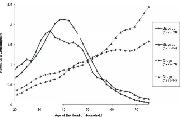
Figure 1. Age profile for the consumption of bicycles and drugs.This figure displays a kernel regression of normalized household consumption for each good as a function of the age of the head of household. The regression uses an Epanechnikov kernel and a bandwidth of 5 years. Each line for a specific good uses an age-consumption profile from a different consumption survey. Expenditures are normalized so that the average consumption for all ages is equal to one for each survey-good pair.
A.2. Age Patterns in Consumption
We use data from the Survey of Consumer Expenditures, 1972–1973 and the 1983 to 1984 cohorts of the ongoing Consumer Expenditure Survey to esti-mate the age patterns in consumption. We cover all major expenditures on final goods included in the survey data. The selected level of aggregation attempts to distinguish goods with different age-consumption profiles. For example, within the category of alcoholic beverages, we separate beer and wine from hard liquor expenditures. Similarly, within insurance we distinguish among health, prop-erty, and life insurance expenditures.
InFigure 1, we present the age profile for two goods using kernel regressions
of household annual consumption on the age of the head of household.9Figure 1
plots the normalized expenditure on bicycles and drugs for the 1972 to 1973 and 1983 to 1984 surveys.10Across the two surveys, the consumption of bicycles peaks between the ages of 35 and 45. At these ages, the heads of household are most likely to have children between the ages of 5 and 10. The demand
9We use an Epanechnikov kernel with a bandwidth of 5 years of age for each consumption good
and survey year.
10For each survey-good pair, we divide age-specific consumption for goodkby the average
for drugs, in contrast, is increasing with age, particularly in the later survey. Older individuals demand more pharmaceutical products.
This evidence on age patterns in consumption supports three general state-ments. First, the amount of consumption for each good depends significantly on the age of the head of household. Patterns of consumption for most goods are not flat with respect to age. Second, these age patterns vary substantially across goods. Some goods are consumed mainly by younger household heads (child care and toys), some by heads in middle age (life insurance and cigars), and others by older household heads (cruises and nursing homes). Third, the age profile of consumption for a given good is quite stable across time. For example, the expenditure on furniture peaks at ages 25 to 35, regardless of whether we consider the 1972 to 1973 or the 1983 to 1984 cohort. Taken as a whole, the evidence suggests that changes in age structure of the popula-tion have the power to influence consumppopula-tion demand in a substantial and consistent manner.
A.3. Demand Forecasts
We combine the estimated age profiles of consumption with the demographic forecasts in order to forecast demand for different goods. For example, consider a forecast of toys consumption in 1985 made as of 1975. For each age group, we multiply the forecasted cohort sizes for 1985 by the age-specific consumption of toys estimated on the most recent consumption data as of 1975, that is, the 1972 to 1973 survey. Next, we aggregate across all the age groups to obtain the forecasted total demand for toys for 1985.
In Table I, we present summary statistics on the consumption forecasts.
Columns 2 and 4 present the 5-year predicted growth rate due to demographics,
cˆk,t+5,t,t−1=ln ˆCk,t+5|t−1−ln ˆCk,t|t−1, for years t=1975 andt=2000,
respec-tively. The bottom two rows present the mean and standard deviation across goods for this measure. In each case, information from the most recent con-sumer expenditure survey is used. In 1975, the demand for child care and toys is low due to the small size of the “Baby Bust” generation. The demand for most adult-age commodities is predicted to grow at a high rate (1.5% to 2% per year) due to the entry of the “Baby Boom” generation into prime consumption age. In 2000, the demand for child-related commodities is relatively low. The aging of the Baby Boom generation implies that the highest forecasted demand growth is for goods consumed later in life, such as cigars, cosmetics, and life insurance.
A.4. Demographic Industries
Table I
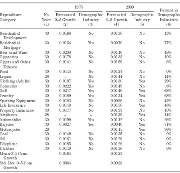
Summary Statistics for Predicted Demand Growth Rates
The table provides a complete list of expenditure categories, with number of years of data avail-ability (Column 1), the average predicted 5-year demand growth rate due to demographic changes in 1975 (Column 2), and the analogous average demand growth rate in 2000 (Column 4). The last two rows present the mean and standard deviation of the 5-year predicted consumption growth across all the goods in the relevant year. This table also indicates whether the industry belongs to the subsample of Demographic Industries in 1975 (Column 3) and in 2000 (Column 5). Each year the subset of Demographic Industries includes the 20 industries with the highest standard deviation of forecasted annual consumption growth over the next 15 years. The percentage of the years 1974 to 2004 in which the expenditure category belongs to the subsample of Demographic Industries is reported in the last column (Column 6).
1975 2000
Percent in Expenditure No. Forecasted Demographic Forecasted Demographic Demographic Category Years 0–5 Growth Industry 0–5 Growth Industry Industries
(1) (2) (3) (4) (5) (6)
Child Care 30 0.0001 Yes 0.0024 Yes 100%
Children’s Books 28 – – 0.0077 Yes 93%
Children’s Clothing 30 0.0226 Yes 0.0138 Yes 100%
Toys 30 0.0044 Yes 0.0084 No 77%
Books—college text books
30 0.0270 Yes 0.0156 Yes 100%
Books—general 30 0.0205 Yes 0.0103 No 84%
Books— K-12 school books
30 –0.0087 Yes 0.0092 Yes 100%
Movies 30 0.0232 Yes 0.0118 No 26%
Newspapers 30 0.0174 No 0.0140 No 0%
Magazines 30 0.0206 Yes 0.0122 No 29%
Cruises 28 – – 0.0143 No 28%
Dental Equipment 30 0.0138 No 0.0133 No 35%
Drugs 30 0.0167 No 0.0153 Yes 10%
Health Care (Services)
30 0.0173 No 0.0135 No 0%
Health Insurance 30 0.0168 No 0.0142 Yes 16%
Medical Equipment 30 0.0173 No 0.0135 No 0%
Funeral Homes and Cemet.
28 – No 0.0166 Yes 59%
Nursing Home Care 30 0.0198 Yes 0.0113 Yes 87%
Construction Equipment
30 0.0200 Yes 0.0121 Yes 100%
Floors 30 0.0177 No 0.0140 Yes 81%
Furniture 30 0.0201 Yes 0.0105 No 58%
Home Appliances
Housewares 30 0.0192 Yes 0.0138 Yes 58%
Linens 30 0.0170 No 0.0130 No 52%
Residential Construction
30 0.0200 Yes 0.0121 Yes 100%
Table I—Continued
1975 2000
Percent in Expenditure No. Forecasted Demographic Forecasted Demographic Demographic Category Years 0–5 Growth Industry 0–5 Growth Industry Industries
(1) (2) (3) (4) (5) (6)
Cigarettes 30 0.0178 No 0.0133 No 10%
Cigars and Other Tobacco
30 0.0141 No 0.0159 No 6%
Food 30 0.0145 No 0.0127 No 0%
Liquor 28 – No 0.0144 No 14%
Clothing (Adults) 30 0.0197 Yes 0.0130 Yes 29%
Cosmetics 30 0.0222 Yes 0.0149 No 6%
Golf 30 0.0217 Yes 0.0146 Yes 68%
Jewelry 30 0.0189 Yes 0.0134 Yes 68%
Sporting Equipment 30 0.0183 No 0.0096 No 42%
Life Insurance 30 0.0140 No 0.0150 Yes 48%
Property Insurance 30 0.0177 No 0.0133 No 10%
Airplanes 28 – – 0.0139 Yes 14%
Automobiles 30 0.0199 Yes 0.0112 No 26%
Bicycles 30 0.0027 Yes 0.0040 Yes 71%
Motorcycles 28 – – 0.0115 Yes 76%
Coal 30 0.0149 No 0.0135 No 0%
information available at timet−1 to identify the goods for which demographic shifts are likely to have the most impact. For each year t and industry k, we compute the standard deviation of the 1-year demand growth forecasts for the next 15 years given bycˆk,t+s+1,t+s,t−1=ln ˆCk,t+s+1|t−1−ln ˆCk,t+s|t−1for
s=0,1, . . . ,15.We define the set of Demographic Industries11in each year t
as the 20 industries with the highest standard deviation of demand growth. In these industries, the forecasted aging of the population induces different de-mand shifts at different times in the future, enabling the estimation of investor horizon.Table Ilists all industries and indicates which industries belong to the subset of demographics industries in 1975 (Column 3) and 2000 (Column 5).
11Ideally, we would like to select industries in which demographics is a better predictor of
-8
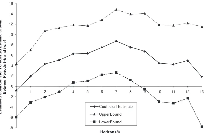
Figure 2. Return predictability coefficient from demand forecasts at different hori-zons.This figure displays the estimated coefficient for each horizon from a univariate OLS re-gression of abnormal returns att+1 on forecasted demand growth betweent+handt+h+1 for the subsample of Demographic Industries during the period 1974 to 2004. The confidence inter-vals are constructed using standard errors clustered by year and then scaled by a function of the autocorrelation coefficient estimated from the sample orthogonality conditions.
Column 6 summarizes the percentage of years in which an industry belongs to the Demographic Industries subsample. The Demographic Industries are associated with high demand by children (child care, toys) and young adults (housing).
A.5. Return Predictability
The evidence supporting return predictability (from DellaVigna and Pollet
(2007)) is summarized inFigure 2. This figure plots the coefficient of univariate
regressions of abnormal annual industry stock returns in yearton forecasted demand growth due to demographics in year t+h. The panel regression in-cludes up to 48 industries during the years 1974 to 2004. AsFigure 2shows, while contemporaneous demand shifts (h equals 1 or 2) do not significantly forecast stock returns, demand shifts 5 to 10 years ahead (hequals 5 to 10) sig-nificantly predict returns.12We interpret this result as evidence that investors
neglect forecastable determinants of fundamentals that are more than 5 years
in the future. The abnormal return for an industry increases when inattentive investors incorporate the upcoming demand shift 5 years in the future.
B. Equity and Debt Issuance
B.1. IPOs
The first measure of equity issuance captures the decision of firms in an industry to go public and is the share of traded companies in industrykand yeartthat are new equity listings in yeart.This measure is available for the full sample (1974 to 2004) for the large majority of industries and ranges from 0.011 (Books: College Texts) to 0.126 (Cruises). As an alternative measure, we also use the share of companies in industrykand yeartthat undertake an IPO according to data from Jay Ritter, though this information is available only from 1980 until 2003. During the sample in which both measures exist, the correlation is 0.8228.
B.2. Net Equity Issuance
The measures of equity issuance for public companies in yeartand industry kare based on net equity issuance in yeartscaled by industry book value of assets in year t−1 (Frank and Goyal (2003)). The measures are available for the entire sample period for most industries, even though the number of companies in an industry is smaller than for the IPO measure, given the additional requirement that the company be in Compustat as well as CRSP. The measure of substantial equity issuance is the fraction of companies in industrykfor yeartthat have net equity issuance greater than 3% of the book value of assets. This threshold, albeit arbitrary, allows us to eliminate equity issues that are part of ordinary transactions, such as executive compensation. The mean of this variable is 0.108, with a standard deviation of 0.190. Similarly, the measure of substantial equity repurchases is the fraction of companies in industry k for year t that have net equity repurchases greater than 3% of the book value of assets. The mean of this variable is 0.067, with a standard deviation of 0.164.
B.3. Net Debt Issuance
The measures of debt issuance for public companies in yeartand industryk are based on the net long-term debt issuance in yeartscaled by industry book value of assets in yeart−1. The measures of substantial debt issuance and substantial debt repurchases follow the same approach described for equity issuance.
III. Empirical Analysis
A. Baseline Specification
tot+10 (the distant future):
Since the consumption growth variables are scaled by 5, the coefficients δ0
andδ1represent the average increase in issuance for one percentage point of
additional annualized growth in demographics at the two different horizons. The fourth subscript indicates that the forecasts of demand growth fromt to t+5 and fromt+5 tot+10 only use information available in periodt−1. The specification controls for market-wide patterns in equity issuance,em,t+1, and
the industry market-to-book ratio,mbk,t+1.13
In this panel setting, the errors from the regression are likely to be corre-lated across industries and over time because of persistent shocks that affect multiple industries. We allow for heteroskedasticity and arbitrary contempo-raneous correlation across industries by clustering the standard errors by year. In addition, we correct these standard errors to account for autocorrelation in the error structure.14
Let X be the matrix of regressors, θ be the vector of parameters, and
ε be the vector of errors. The panel has T periods and K industries. Under the appropriate regularity conditions, 1/T( ˆθ−θ) is asymptotically distributed N(0,(X′X)−1S(X′X)−1), where S=Ŵ
0+∞q=1(Ŵq+Ŵq′) and Ŵq=
E[(kK=1Xk,tεk,t)′(kK=1Xk,t−qεk,t−q)]. The matrix Ŵ0 captures the
contempora-neous covariance, whereas the matrix Ŵq captures the covariance structure between observations that areqperiods apart. Although we do not make any as-sumptions about contemporaneous covariation, we assume that X′
k,tεk,tfollows
an autoregressive process given byX′
k,tεk,t=ρX′k,t−1εk,t−1+η′k,t, whereρ <1 is
a scalar and E[(Kk=1Xk,t−qεk,t−q)′(kK=1ηk,t)]=0 for anyq>0.
These assumptions implyŴq=ρqŴ0, and therefore, S=[(1+ρ)/(1−ρ)]Ŵ0. The full derivation and details are inDellaVigna and Pollet (2007). The higher the autocorrelation coefficientρ,the larger the terms in the matrixS. SinceŴ0
andρare unknown, we estimateŴ0with 1 T
T
t=1X
′
tεtˆεˆ′tXtwhereXtis the matrix
of regressors and ˆεtis the vector of estimated residuals for each cross-section.
We estimate ρ from the pooled regression for each element of X′
k,tεˆk,t on the
respective element ofX′
k,t−1εˆk,t−1.
We use the set of Demographic Industries for the years 1974 to 2004 as the baseline sample. As discussed earlier, these industries are more likely to be affected by demographic shifts.
13Including lagged profitability and lagged investment does not affect the results (seeTable IV). 14This method is more conservative than clustering by either industry or year. In the empirical
B. IPO Results
InTable II, we estimate the regression specification given byequation (9)for
the share of new equity listings. In the specification without industry or year fixed effects (Column 1), the impact of demographics on new equity listings is identified by both between- and within-industry variation in demand growth. The coefficient on short-term demographics, ˆδ0=3.35, is marginally signifi-cantly different from zero, whereas the coefficient on long-term demographics, ˆ
δ1= −4.84, is significantly different from zero. When we introduce controls for the industry market-to-book ratiombk,tand for the aggregate share of new
listingsem,t(Column 2) the impact of long-term demographics attenuates to a
marginally significant ˆδ1= −2.49 and the effect of short-term demographics
be-comes insignificant.15If we include industry fixed effects (Column 3), demand
growth in the near future has a marginally significant positive effect on the share of new listings (ˆδ0=2.45), whereas demand growth in the further future
has a significant negative effect (ˆδ1= −3.07). We obtain similar results if we
include year fixed effects (Column 4). In this specification, the identification depends on within-industry variation in demand growth after controlling for common time-series patterns.16
For the specifications in Columns 2 through 4, a 1% annualized increase in demand from year t to t+5 increases the share of net equity issues by about 2.5 percentage points from an average of 6.33 percentage points. A one percentage point increase in demand growth corresponds approximately to 1.7 standard deviations.17A one percentage point annualized increase in demand from yeart+5 tot+10 decreases the share of net equity issues by about three percentage points, a significant and economically large effect. Although this effect is large, we note that a decrease of half a percentage point is inside the confidence interval for the coefficient estimate.
In Columns 5 and 6, we use the alternative measure based on the share of IPOs according to data from Jay Ritter. We again find that long-term de-mand growth due to demographics is negatively related to the share of IPOs. While the coefficient estimate is positive for short-term demand growth due to demographics, this effect is not significant.
Finally, in Columns 7 and 8 we present the results for the benchmark mea-sure of IPOs, but for the sample of Nondemographic Industries. The coefficient estimates are similar but the standard errors are about twice as large, despite the higher number of observations. For this set of industries, the demographic shifts are not important enough determinants of demand, and hence the esti-mates are noisy. Notice that the limited variation in the independent variable does not per se lead to biases in the estimated coefficient. If we group the two
15In this and the subsequent specifications inTable II, the estimate ofρis approximately 0.17,
resulting in a proportional correction for the standard errors of(1+ρˆ)/(1−ρˆ)=1.19.
16We find quantitatively similar results using the Fama–MacBeth regression methodology (see
the Internet Appendix).
17For this sample, the mean forecasted annualized demand growth fromttot+5 (t+5 to
Capital
Budgeting
v
ersus
Market
T
iming
255
Predictability of New Equity Listings Using Demographics
Columns 1 through 4 report the coefficients of OLS regressions of the share of firms in an industry that are new listings in CRSP for yeart+1 on the forecasted annualized demand growth due to demographics betweentandt+5 and betweent+5 andt+10 for the subset of Demographic Industries. Columns 5 and 6 report regression results for the subset of Demographic Industries where the dependent variable is defined using new listings recorded in Jay Ritter’s IPO sample (from 1980 until 2003). Columns 7 and 8 report the regression coefficients for the subset of Nondemographic Industries. The forecasts are made using information available as of yeart–1. The forecasts of demand growth are annualized using the number of years in the forecast (five for each forecast). Each year the subset of Demographic Industries includes the 20 industries with the highest standard deviation of forecasted annual consumption growth over the next 15 years. Standard errors, reported in parentheses, are clustered by year and then scaled by a function of the autocorrelation coefficient estimated from the sample orthogonality conditions. A thorough description of the standard errors is available in the text (∗significant at 10%;∗∗significant at 5%;∗∗∗significant at 1%).
Share of Firms That Are New Equity Listings
Dependent Variable Demographic Nondemographic
Industry Sample
(1) (2) (3) (4) (5) (6) (7) (8)
Forecasted annualized demand 3.349 2.237 2.446 2.785 1.994 2.831 1.687 –0.525 growth betweentandt+5 (1.847)∗ (1.474) (1.270)∗ (1.304)∗∗ (1.877) (2.273) (2.866) (4.502) Forecasted annualized demand –4.843 –2.486 –3.071 –3.153 –4.793 –3.572 –4.955 –6.930
growth betweent+5 andt+10 (1.453)∗∗∗ (1.384)∗ (1.403)∗∗ (1.360)∗∗ (1.949)∗∗ (1.913)∗ (3.289) (4.270)
Industry market-to-book ratio 0.000 0.003 0.004 0.006 0.002 0.004 0.011
(0.0065) (0.007) (0.010) (0.009) (0.012) (0.009) (0.009)
Aggregate share of new listings 0.890 0.841 1.229 0.716
(0.143)∗∗∗ (0.151)∗∗∗ (0.1507)∗∗∗ (0.072)∗∗∗
Industry fixed effects X X X X X X
Year fixed effects X X X
Jay Ritter’s IPO sample X X
R2 0.040 0.133 0.245 0.306 0.260 0.315 0.264 0.297
samples together and consider all industries, the results are slightly stronger than those for the Demographic Industries sample.
To summarize, the impact of demand shifts on the share of new equity list-ings depends on the horizon of the demand shifts. Demand shifts occurring in the near future increase the share of IPOs, consistent with capital budgeting, although this effect is not always significant. In contrast, demand shifts occur-ring further in the future significantly decrease the share of IPOs, consistent with market timing. In both cases, the effect is economically large.
C. Net Equity Issuance Results
InTable III, we estimate the effect of demand shifts on net equity issuance
by existing firms in the sample of Demographic Industries.18 In Columns 1 through 3, we use the share of companies in an industry with net issuance above 3% of assets as the measure of large equity issues. In the specification without industry or year fixed effects (Column 1), the coefficient on short-term demographics is positive but insignificant (ˆδ0=4.05), whereas the coefficient
on long-term demographics is significantly negative (ˆδ1= −7.24 ). When we
in-troduce the controls for the industry market-to-book ratiombk,t+1and aggregate
net equity issuanceem,t+1as well as industry fixed effects (Column 2), the
coef-ficient estimates for both the short-term and the long-term demographics are statistically significant.19Introducing year fixed effects (Column 3) lowers the
coefficient on short-term demographics considerably, rendering it insignificant. In Columns 4 through 6, we present the results for large equity repurchases, that is, the share of companies in an industry with net repurchases above 3% of assets. As predicted, the qualitative results are of the opposite sign compared to the estimates for large equity issuance. However, the estimates are less precisely estimated. Near-term demographic shifts are not significantly related to repurchases. Long-term demographic shifts increase repurchases in Columns 4 and 5 but not in Column 6.
In Columns 7 and 8, we analyze the continuous measure of net equity is-suance. We find that near-term demographic shifts increase net equity issuance and long-term demographic shifts decrease net equity issuance. In the Internet Appendix, we revisit the specifications in Columns 7 and 8 using an alterna-tive measure of net equity issuance in the spirit ofBaker and Wurgler (2002), defined as the change in book equity minus the change in retained earnings (scaled by lagged assets), and the results are qualitatively similar.
To summarize, the evidence matches the predictions of the model and is consistent with the findings for new listings, providing support for both capital budgeting and market timing.
18The results are qualitatively similar but highly imprecisely estimated for the sample of
Non-demographic Industries.
19In this and the subsequent specifications in Table VI, the estimate ofρvaries between zero
and 0.30, for an average of 0.15, resulting in a proportional correction for the standard errors of
Capital
Budgeting
v
ersus
Market
T
iming
257
Predictability of Net Equity Issuance and Net Equity Repurchases Using Demographics
Columns 1 through 3 report the coefficients of OLS regressions of the share of firms in an industry with stock issues minus stock repurchases divided by the lagged book value of assets that is greater than 3% for yeart+1 on the forecasted annualized demand growth due to demographics betweentandt+5 and betweent+5 andt+10. Columns 4 through 6 report regression coefficients of the share of firms in an industry with stock repurchases minus stock issues divided by the lagged book value of assets that is greater than 3% for yeart+1 on the forecasted annualized demand growth. Columns 7 and 8 report regression coefficients of industry stock issues net of stock repurchases scaled by industry book value of assets (a continuous measure) for yeart+1 on the forecasted annualized demand growth. The demand forecasts are made using information available as of yeart– 1. The forecasts of demand growth are annualized using the number of years in the forecast (five for each forecast). All specifications only include observations from the subset of Demographic Industries, which are the 20 industries with the highest standard deviation of forecasted annual consumption growth over the next 15 years. Standard errors, reported in parentheses, are clustered by year and then scaled by a function of the autocorrelation coefficient estimated from the sample orthogonality conditions. A thorough description of the standard errors is available in the text (∗significant at 10%;∗∗significant at 5%;∗∗∗significant at 1%).
Large Net Equity Issues Large Net Equity Repurchases Net Equity Issuance Dependent Variable
(1) (2) (3) (4) (5) (6) (7) (8)
Forecasted annualized demand 4.046 4.564 2.304 –4.209 –1.688 –0.939 2.529 1.782 growth betweentandt+5 (2.539) (1.955)∗∗ (1.637) (1.839)∗∗ (1.357) (1.619) (0.9970)∗∗ (0.821)∗∗ Forecasted annualized demand –7.241 –5.267 –4.294 3.080 3.699 3.222 –2.852 –1.533
growth betweent+5 andt+10 (2.588)∗∗∗ (2.170)∗∗ (2.013)∗∗ (1.760)∗ (1.859)∗∗ (2.070) (1.034)∗∗∗ (1.048)
Industry market-to-book ratio 0.016 0.037 0.056 0.046 0.010 0.012
(0.021) (0.023) (0.016)∗∗∗ (0.019)∗∗ (0.007) (0.009)
Aggregate share of large 0.892
net equity issues (0.125)∗∗∗
Aggregate share of large 1.047
net equity repurchases (0.353)∗∗∗
Aggregate net equity issuance 2.557
(0.677)∗∗∗
Industry fixed effects X X X X X X
Year fixed effects X X X
R2 0.030 0.284 0.349 0.013 0.169 0.213 0.230 0.286
D. Combined Issuance Results
Since the model does not distinguish between the two forms of equity issuance (and the results are consistent across the two), we introduce a combined mea-sure of equity issuance. This meamea-sure provides additional power and reduces the number of specifications in the subsequent analysis. The combined measure is the average of the IPO measure (Columns 1 through 4 ofTable II) and the large equity issuance measure (Columns 1 through 3 ofTable III). The results for the combined measure of equity issuance are presented in Table IV and match the findings for each of the constituent measures (Columns 1 through 3
ofTable IV).
The improved statistical power associated with the combined measure leads to a more consistent rejection of the null hypothesis for both short-term and long-term demographic shifts. In Columns 4 through 6, we provide evidence regarding the appropriateness of the standard errors employed in the paper. In particular, we replicate the regressions in the first three columns using the double-clustering procedure described by Thompson (2011). In most regres-sions, the standard errors for the coefficient on long-term demand growth are more conservative using our approach than those using the double-clustering procedure.
In the last two columns of Table IV, we introduce additional controls for lagged accounting return on equity and lagged investment. Neither of these control variables has an appreciable impact on the point estimates or standard errors of the coefficients for short-term or long-term demand growth. We do not use these controls in the benchmark specifications because they are themselves affected by demographic shifts: investment should be endogenously related to investment opportunities (and perhaps mispricing), and profitability is related to demand shifts as documented inDellaVigna and Pollet (2007).
E. Graphical Evidence
Using the combined issuance measure, we present graphical evidence on how equity issuance responds to demographic shifts at different time horizons. For each horizonh∈ {0,13}, measured in years, we estimate
ek,t+1=λ+δH[ˆck,t+h+1|t−1−cˆk,t+h|t−1]+βmem,t+1+βbmbk,t+1+ηk+εk,t (10)
for the sample of Demographic Industries. The coefficientδHmeasures the
ex-tent to which demand growth h years ahead forecasts stock returns in year t+1. The specification controls for market-wide patterns in issuance, as cap-tured by em,t+1, for industry market-to-book, as captured by mbk,t+1, and for
Capital
Budgeting
v
ersus
Market
T
iming
259
Predictability of Combined Equity Issuance Using Demographics
Columns 1 through 8 report the coefficients of OLS regressions of the share of companies in an industry that issued equity either through a new listing in CRSP or through a seasoned issuance for yeart+1 on the forecasted annualized demand growth due to demographics betweentandt+5 and betweent+5 andt+10. The forecasts are made using information available as of yeart–1. The forecasts of demand growth are annualized using the number of years in the forecast (five for each forecast). All specifications only include observations from the subset of Demographic Industries, which are the 20 industries with the highest standard deviation of forecasted annual consumption growth over the next 15 years. Columns 1 through 3 report standard errors, reported in parentheses, are clustered by year and then scaled by a function of the autocorrelation coefficient estimated from the sample orthogonality conditions. A thorough description of these standard errors is available in the text. Columns 4 through 6 report standard errors based on the double-clustering approach recommended by Thompson (2011). Levels of statistical significance are as follows:∗significant at 10%;∗∗significant at 5%;∗∗∗significant at 1%.
Share of Firms That Are New Listings or Conducted a Large Net Equity Issuance Dependent Variable
(1) (2) (3) (4) (5) (6) (7) (8)
Forecasted annualized demand 3.717 3.509 2.564 3.717 3.509 2.564 3.194 2.436 growth betweentandt+5 (2.250)∗ (1.506)∗∗ (1.247)∗∗ (1.741)∗∗ (1.691)∗∗ (1.802) (1.363)∗∗ (1.168)∗∗ Forecasted annualized demand –6.103 –3.907 –3.749 –6.103 –3.907 –3.749 –3.674 –3.519
growth betweent+5 andt+10 (2.052)∗∗∗ (1.571)∗∗ (1.517)∗∗ (1.863)∗∗∗ (1.476)∗∗ (1.345)∗∗∗ (1.477)∗∗ (1.412)∗∗
Industry market-to-book ratio 0.009 0.021 0.009 0.021 0.006 0.014
(0.011) (0.012)∗ (0.011) (0.014)∗ (0.011) (0.012)
Industry investment –0.032 –0.023
(0.034) (0.032)
Industry accounting return on 0.117 0.141
equity (0.047)∗∗ (0.050)∗∗∗
Aggregate combined equity issues 0.947 0.947 0.974
(0.134)∗∗∗ (0.148)∗∗∗ (0.135)∗∗∗
Industry fixed effects X X X X X X
Year fixed effects X X X
Double clustering X X X
R2 0.046 0.349 0.413 0.046 0.349 0.413 0.359 0.426
-8
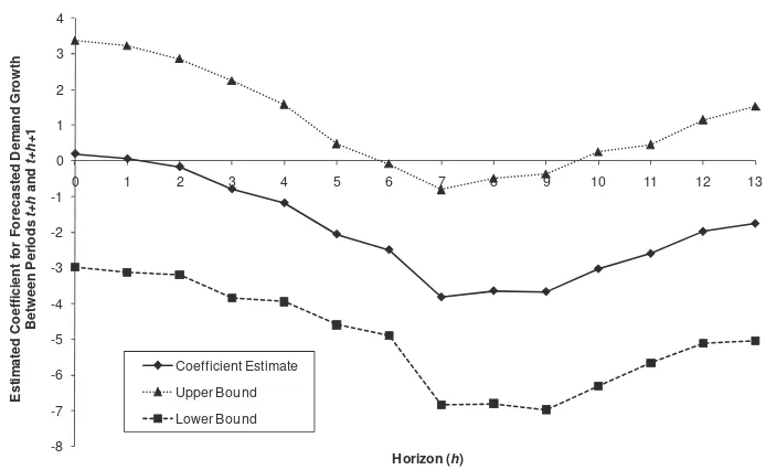
Figure 3. Combined equity issuance predictability coefficient from demand forecasts at different horizons.This figure displays the estimated coefficient for each horizon from an univariate OLS regression of the share of companies in an industry that issued equity either through a new listing in CRSP or through a seasoned issuance for yeart+1 on forecasted demand growth betweent+handt+h+1 for the subsample of Demographic Industries during the period 1974 to 2004. Each regression includes controls for market-wide patterns in new listings, industry-level book-to-market, and industry fixed effects. The confidence intervals are constructed using standard errors clustered by year and then scaled by a function of the autocorrelation coefficient estimated from the sample orthogonality conditions.
Figure 3presents the result from the estimation of (10) for different horizons.
Demand growth due to demographics from 0 to 1 year ahead is associated with a small (insignificant) increase in IPOs according to the benchmark measure. Demand growth due to demographics 2 or more years ahead, in contrast, has a negative impact on IPO issuance. The impact is most negative (and statistically significant) for demand shifts 7 to 9 years ahead. Demographic shifts more than 10 years in the future have a smaller (though still negative) impact on IPO decisions.
F. Time-to-Build
The model indicates that the impact of both long-term and short-term de-mographics should be attenuated by time-to-build. The investment required to expand production in response to future demographic demand could take several years, possibly in excess of the 5 years that the proxy for short-term demand allows. In this case, the lengthy time-to-build will attenuate the nega-tive relationship between long-term demand due to demographics and security issuance. Essentially, long-term demand captures not only the market timing (which induces a negative relation), but also capital budgeting (which induces a positive relation). In addition, in the presence of substantial time-to-build, short-term demand is unrelated to equity issuance because it is difficult to build additional capacity quickly enough to take advantage of a positive de-mand shift.
To provide evidence on the importance of time-to-build,we use as a proxy of time-to-build the amount of work in progress (Compustat data item 77) divided by the book value of the firm. Firms that have a higher share of work in progress are more likely to have a lengthy production process and greater difficulty adjusting capacity rapidly.20 We split observations in two groups,
above and below the median value of 0.005.
We present the results in Columns 1 through 4 ofTable V. We find that, for the high time-to-build industries (Columns 1 and 2), both coefficient estimates are closer to zero and not statistically significant. For the low time-to-build industries (Columns 3 and 4), the coefficient estimates are larger (in abso-lute value) than those for the benchmark sample, and long-term demand is statistically significant. Therefore, time-to-build appears to affect the response to demand shifts in a manner consistent with the predictions of the model.
G. Industry Concentration
The impact of a demand shift on equity issuance could depend on the market structure. In a perfectly competitive industry, there is no impact on abnormal profitability, and hence, no possibility of mispricing associated with long-term demand shifts. At the other extreme, a monopolist generates abnormal prof-its from a positive demand shift, and therefore, demand in the distant future generates mispricing in the presence of limited attention. Thus, evidence of market timing should be more substantial for industries with high market
20We thank Kenneth French for suggesting work in progress as a measure of time-to-build. The