316
15
and Oligopoly
C O N C E P T S
● Monopolistically Competitive Market ● Product Differentiation
● Excess Capacity Theorem ● Advertising or Selling Costs
● Persuasive Advertisement ● Informative Advertisement
● Oligopoly ● Duopoly
● Kinked Demand Curve Model ● Cournot Model
● Best Response Curve ● Bertrand Model
P
erfect competition and monopoly are the two extreme forms of market structure. The former has infinitely many firms producing a homogeneous product with the implication that any particular firm has no market power and behaves as a price taker. The latter has only one firm.In this chapter we study monopolistic competition and oligopoly, which are intermediate between perfect competition and monopoly.
MONOPOLISTIC COMPETITION
This market structure has the following features: (a) There are a large number of sellers and buyers. (b) There is free entry and exit in the long run. (c) Moreover, there is product differentiation. That is, each firm produces a brand or variety (of the same product) that is unique, that is, different from what any other firm pro-duces. The varieties produced are very close substitutes of one another. Products like toothpaste, soap and lipstick are good examples.1Service providers like tai-lors who make suits and fancy hair-cut salons are also good examples; each of these basically provides the same service, yet each one is slightly different from the other in terms of style, feel and look.
The features (a) and (b) respectively imply that each firm is small relative to the market and earns zero abnormal profits in the long run. Thus (a) and (b) are com-petitive features. However, (c) is a monopoly feature in the sense that any given brand is produced only by one firm; hence each firm has some monopoly power. Put differently, product differentiation confers some market power to a monopoli-stically competitive firm, even though it is small compared to the entire market. Monopolistic competition is thus a market form that has monopolistic and com-petitive features.
Equilibrium in the Short Run
The monopoly feature implies that a monopolistically competitive firm also faces ARand MR curves for its brand and it maximises profits at the level of output, where MR=MC. It charges a price, which exceeds marginal cost.
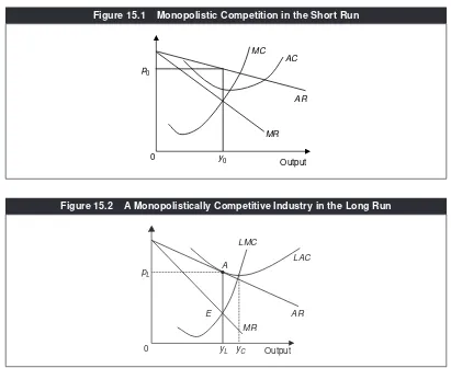
Analytically, all these are analogous to monopoly, except for one qualitative dif-ference. That is, since there are close substitutes available for any particular brand, the demand curve facing a monopolistically competitive firm (unlike that facing a monopoly firm) is very elastic, implying that the AR curve must be quite flat. Figure 15.1 draws a short-run situation of a representative firm in monopolistic competition. The AR curve is relatively flat. The MR curve corresponds to the ARcurve. The firm maximises where MR equals MC, producing the amount y0 and charging price p0.
Long-run Equilibrium
There is, however, a major difference between monopolistic competition and monopoly in the long run. Unlike in monopoly, there is free entry and exit, imply-ing that abnormal profit is driven to zero. This is equivalent to P=LAC, where the letter ‘L’ refers to the long run. Together with the profit-maximising condition
MR=LMC, we can then compactly write the long-run equilibrium conditions in monopolistic competition as:
MR=LMC;
P=LAC.
Figure 15.2 illustrates the long-run equilibrium. Mark that at the point where
MR= LMC, ARis also equal to LAC; therefore profits are zero. The representative firm produces output yLand charges price pL.
Even though the long-run profits are zero, the situation is not exactly analogous to the long-run, competitive equilibrium. Notice in Figure 15.2 that whereas under
AC
AR
MR p0
MC
0
Output y0
Figure 15.1 Monopolistic Competition in the Short Run
LAC LMC
AR MR
0
A
Output E
pL
yC
yL
perfect competition, a firm would have produced at the minimum point of the long-run average cost (that is, at yC), in monopolistic competition, the equilibrium output lies to the left of where the LACis minimised—such as at yL. That is, under monopolistic competition, in the long run there are increasing returns to scale and unit cost is not minimised. In microeconomic theory this result is known as the excess capacity theorem in the sense that in equilibrium, the production is not optimised from the viewpoint of using up all economies of scale without stepping into the range of diseconomies of scale.
Social Welfare Implications
The excess capacity theorem means that each firm in the industry is so small that it is not able to fully exploit scale economies till they are exhausted. In other words, compared to the social optimum (which takes into account production efficiency), there are ‘too many’ firms, implying that each firm is ‘too small’. While this is a source of welfare ‘loss’, compared to the social optimum, it provides a welfare gain of a kind we have not discussed so far.
Suppose society positively values the variety available to a consumer. Compare a situation where you walk into a garment shop and find men’s shirts of three colours to another where you find men’s shirts of many different colours and combinations. All else the same, you are better off in the latter situation. If so, a large number of firms imply greater variety, which is a source of welfare gain.
Therefore, we cannot generally say whether, compared to the social optimum, the monopolistically competitive equilibrium entails too many or too few firms and varieties. In any event, to the extent that price is not equal to marginal cost implies some welfare loss compared to what is the first-best for the society.
Advertising
Although the features of monopolistic competition are a combination of perfect competition and monopoly, in terms of decision-making, there is one aspect of it, which is different from both perfect competition and monopoly. That is, monop-olistically competitive firms typically engage in advertising, that is, they incur advertising costsor what are also called selling costs. (Remember the concept of advertising elasticity in Chapter 2.) It is because of the need to maintain a percep-tion in the mind of the potential consumers that their respective brands are different (and more tasteful or classy), compared to other brands. This is called per-suasive advertisement and its purpose is to lure away consumers from other brands to your brand. (In perfect competition, the product is perfectly homoge-neous and hence there is no scope to engage in persuasive advertisement. In monopoly, since there is no competition, there is no need to engage in persuasive advertisement.)
which can be potentially used for production; advertising itself is a big industry. Therefore, advertising costs are ‘wasteful’ from the viewpoint of the society.
However, not all advertising costs are wasteful. On many occasions, there is informative advertisement (for example, about health), which is useful for the consumers. Further, even if it is persuasive advertising, an opportunity to advertise may increase competition, reduce prices and thereby improve social welfare. Indeed, a classic study by Lee Benham found that in America the price of eye-glasses was cheaper on the average by $20 (at 1963 prices) in the states that allowed advertising than in the states that did not allow advertising.
OLIGOPOLY
Features
An oligopoly market is one that is inhabited by a limited number of sellers or producers. A special case where there are only two firms is called a duopoly mar-ket. In oligopoly the product may be homogeneous or differentiated. The number of firms being limited means that entry and exit processes are limited. This could be due to government regulations with respect to entry and exit, or the technology, which may involve huge fixed costs, deterring small firms from entering the indus-try or surviving in the market for long.
There are numerous examples of an oligopoly market such as passenger air-crafts, air-conditioners, cars and cellular telephone services.
The most crucial behavioural difference of oligopoly with other market struc-tures studied so far is that each firm in the industry is big enough to hold market power to the extent that a change in the price, advertising or output decision by any one firm significantly affects the profit of any other firm. Put differently, each firm is ‘important’ for any other firm, implying that there is a game-theoretic, strategic interaction among firms. In deciding price, quantity and so on, each firm must take into consideration the effects of its own action on the actions to be chosen by others and vice versa. Whether the product is homogenous or differentiated does not have any bearing on whether the market is an oligopoly or not. One can talk about a homogeneous-product oligopoly or an oligopoly with product differentiation.
As a result, the analysis of oligopoly is relatively complicated. Unlike perfect competition, monopoly or monopolistic competition, there is no single unified ‘model’ of oligopoly. There are several ‘models’ of oligopoly instead. In what follows, we outline a few of them.
Kinked Demand Curve Model
one minute to the next, whereas the former are relatively stable. The price stability in an oligopoly market is explained by the kinked demand curve analysis.
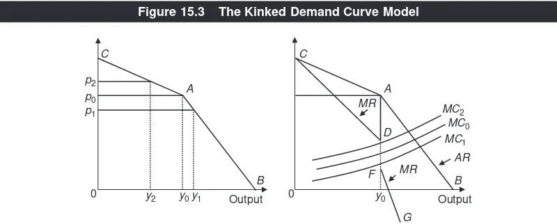
Consider an oligopoly industry in which the firms produce a differentiated product. Think of a particular firm, say firm X, which is initially producing y0and charging the price p0. This quantity-price combination is shown at the point Ain the left panel of Figure 15.3. Starting from this initial situation, suppose that the firm cuts its price, say to p1. Will the other firms ‘keep quiet’ and not change their prices? No, because if they do, they will lose customers to firm X, reducing their profits. Their optimal response will be to lower prices too. Thus, the firm initiat-ing the price cut (firm X) will gain only a modest increase in sales (to the extent that there is a decline in the price of allbrands, which encourages the consumers to buy more of the product across the board). At p1, the quantity sold by firm Xis marked by y1. The key point is that below the price p0, the demand curve is rela-tively inelastic and steep—reflecting a price-cut response by other firms. This is illustrated by the relatively steep line segment AB.
What happens if firm X, instead of lowering its price, increases it, say to p2? The other firms will not mind this at all as they stand to gain. Since the brand produced by firm X is costlier, it is likely to lose a lot of sales to other firms. That is, the quantity sold by firm Xwill decrease by a relatively large amount—from y0to y2. Hence, above the price p0, the demand curve facing firm Xwill be very elastic (flat). This is indicated by the segment AC.
Combining what happens with a price cut and a price hike, CABis the entire demand curve facing a particular firm X. (The two segments are drawn as straight lines for simplicity only, but they need not be so.) Note the ‘kink’ (sharp edge) at the point A. What is the economic rationale behind such a kink? It is the big difference in the price elasticity along the demand curve on the two sides of the price p0, which arises from the asymmetry in the response of other firms with regard to a price cut and a price rise initiated by a particular firm.
As the demand curve facing a firm is its ARcurve, the line CAB in the left panel of Figure 15.3 is marked as the ARcurve in the right panel. What is the
B
corresponding MRcurve? In the output range from 0 to y0, the MRcurve will have a segment like CDwhich corresponds to the segment CAon the ARcurve. In the output range beyond y0, the MRcurve has the segment FG,corresponding to the segment ABon the ARcurve. Hence, the MRcurve is discontinuous.
Now let the curve MC0denote firm X’s marginal cost curve, passing through the discontinuous part DF. At what level of output is the firm’s profit maximised? The answer is y0 and the reason is as follows. At any level of output below y0,
MR>MC, so that profit can be increased by increasing the output. Similarly, at
any output above y0, MR<MCand, therefore, profit will increase by decreasing
the output. These two statements imply that the profit is the maximum at the out-put level corresponding to the kink.
Given this equilibrium, suppose there is some variation in the cost conditions fac-ing the firm such that the MCcurve shifts to say MC1or MC2. Notice that this has no impact on the firm’s profit-maximising output. It continues to produce at the kink and charge the price p0. In other words, the price chosen by the firm is insensitive to a change in cost conditions—at least to some extent (that is, as long as the MC
curve passes between the points Dand F). This is how the kinked demand curve model explains why price variations are not likely to be large in oligopoly markets. While this model is useful, it has two major deficiencies. First, the model does not explain the position of the kink on the demand curve. It starts with an arbitrarily given output-price combination and then argues that it is the profit-maximisation combination. Second, although it appeals to the notion of strategic interaction (that is, how one firm responds to a change in strategy by another), it is still not grounded in equilibrium concepts in game theory, for example, the Nash equilib-rium as discussed in Chapter 13.
Quantity Competition: The Cournot Model
Cournot, a French economist and mathematician in the 19th century, formulated a model of duopoly competition in quantities produced and sold, which could be founded on the notion of Nash equilibrium and, therefore, is consistent with game theory.2
Let the two firms be called Aand B. Assume that the product is homogeneous. Figure 15.4 depicts the industry demand curve DD. The questions are: (i) what will each firm produce and (ii) what will be the market price? Of course, if we have the answer to question (i), the answer to question (ii) is immediate—add up the two firms’ outputs to get the industry-level output and the equilibrium price is the one at which the total quantity demanded is equal to the industry output. Let yAand yBdenote the output produced and sold by firm Aand firm B respec-tively. For instance, if yA+ yB= Y0, the market price, as shown in Figure 15.4, is p0.3
2The duopoly model is capable of being easily generalised to the case of more than two firms.
3We are not assuming that the market price is p
Recall that Nash equilibrium is defined by a set of strategies chosen by the players such that any single player will not benefit from changing his strategy. In the present context, the players are firms Aand B. The strategies are (the indi-vidual) outputs chosen by the firms. A particular combination of outputs, say (y0
A,yB0), will qualify as a Nash equilibrium if, given yB0, firm Ahas no incentive to
choose any output other than y0
A, that is, the yA0 is the profit-maximising output of
firm Awhen yB= y0
B, and likewise y0B is the profit-maximising output of firm B
when yA=y0
A. How are yA0 and yB0determined?
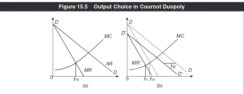
Consider first the profit-maximising behaviour of firm Aat various possible values of yB. Suppose that yB=0. Then firm Ahas the entire market, that is, it is a monopoly. The market demand curve is its ARcurve. Panel (a) of Figure 15.5 illus-trates this. The ARcurve drawn is the same as the demand curve in Figure 15.4. Figure 15.5(a) also depicts the marginal cost curve of firm A. Its profit-maximising output is ym, at which MR= MC. Put differently, at yB= 0, the best response of firmAis to produce output equal to ym.
D 0
D
p0
yBY0
yA
Figure 15.4 Market Price in the Cournot Model
D
MR yB
MC
0 D
0
AR MC
D D′ D
D′
ym y1 ym
(b) (a)
MR′
Now suppose firm Bproduces a small quantity. Then, compared to yB= 0, at any given quantity sold by firm A, the total quantity sold in the market will be higher and hence the market price will be less. That is, the average revenue will be smaller. Thus the ARcurve facing firm Awill lie to the left of its ARcurve when yB=0. This
is shown in the panel (b) of Figure 15.5, which depicts the same market demand curve as in panel (a). The AR curve of firm Ais D’D’, such that the horizontal difference between DD and D’D’ is the amount produced by firm B. The corre-sponding MRcurve is marked by MR’. The associated profit-maximising output by firm Ais equal to y1. This is the best response of firm A.
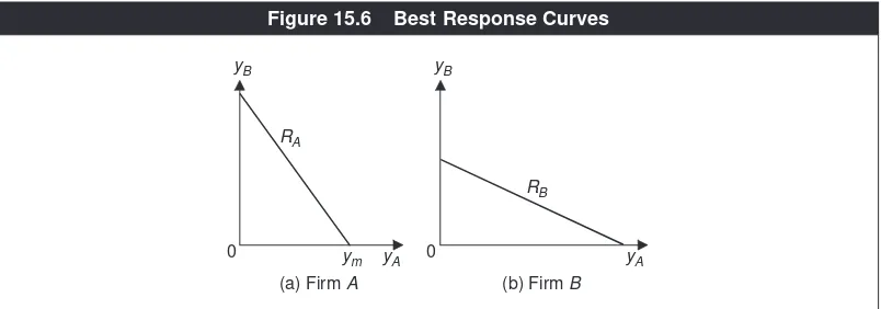
Note that y1is less than ym, that is, a higher output by firm Bimplies a smaller profit-maximising output by firm A. It is because if one firm is able to sell a higher quantity than before, it is equivalent to a decrease in the demand curve facing the other firm. Hence, the other firm produces less in equilibrium. Such reasoning implies that the equilibrium output of firm Adecreases with the output of firm B. This relationship is graphed in Figure 15.6(a). The curve is marked RA, which we can call the best response curve of firm A. In general, the best response curve
shows a player’s best (optimal) strategies corresponding to different strategies chosen by other player(s).
Similarly we can analyse the profit-maximising behaviour of firm Bat various levels of output by firm A. By the same logic, the equilibrium output of firm B
decreases with the output of firm A. This relationship is shown by the RBcurve in Figure 15.6(b). This is the best response curve of firm B.
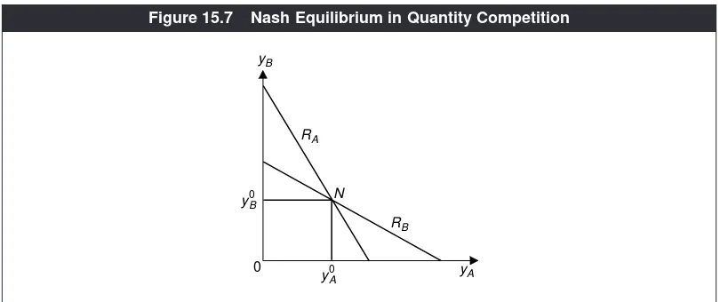
Figure 15.7 graphs the best response curves of the two firms together. Mark the point of intersection, N. This is the equilibrium point, solving the Nash-equilibrium outputs, y0
Aand yB0respectively for firm Aand firm B. Why does the
intersection point constitute Nash equilibrium? The point Nbeing on RAmeans that when yB= y0
B, firm Amaximises its profit by producing yA0 and thus it has no
incentive to choose any output other than y0
A. The point Nalso lies on RB, meaning
that when yA= y0
A, y0Bis the profit-maximising output of firm Band thus firm Bhas
no incentive to choose any output other than y0
B.
(b) Firm B yB
RB
yA
0 yB
ym
RA
0
(a) Firm A yA
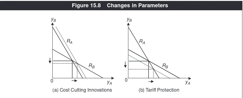
We can now use this quantity-competition framework to determine the effects of changes in ‘parameters’ facing the industry. The term ‘parameter’ here means a basic condition or state of the industry, which is not influenced by the choices made by producers or consumers, but which can change due to extraneous factors. For example, suppose firm Ais able to discover a new way of organising work-ers in the production activity such that its MC curve shifts down. How will it affect the equilibrium quantities produced by both firms? Turn first to Figure 15.5. If the MCcurve shifts down, at any given level of output by firm B(which fixes the position of the MRcurve facing firm A), the intersection of the MRcurve and the new MCcurve will occur at a higher level of output by firm A. In other words, the profit-maximising output of firm Ais higher than before at any given level ofyB. This implies that the RAcurve in Figure 15.6 will shift to the right (but there will be no shift of the RBcurve).
This shift is shown in Figure 15.8(a). In the new (Nash) equilibrium, firm A pro-duces more and firm B produces less. These are reasonable outcomes. A cost reduction method discovered and executed by a firm will enable it to produce more in the market and force its rival to produce less.
Consider another application. In India, steel is sold by Indian and foreign firms. Among Indian firms, SAIL (Steel Authority of India) is the largest, having plants at Rourkela, Durgapur, Bhilai and Bokaro. Tata Iron and Steel Company is also a big manufacturer of steel. However, for analytical purposes, assume that there is one domestic producer of steel. India also imports steel from many countries, on which it imposes an import duty. For the sake of argument, assume that there is only one foreign firm who sells steel in India. Hence, ignoring quality difference between domestic and foreign steel, we can depict the Indian steel market as a duopoly, having a domestic firm and a foreign firm. Note that paying import duty adds to the marginal cost of selling steel in India by the foreign firm. Go back to Figure 15.6 and interpret RAand RBas the best response curves of the domestic
yB
RB
yA RA
N
y0A y0B
0
firm and the foreign firm respectively, keeping in mind that RBtakes into account the tariff cost facing the foreign firm. Using Figure 15.7, in equilibrium, the former sells y0
Aof steel and the latter sells yB0.
Suppose that, starting from a situation of 10 per cent import duty on steel, the Indian government slaps a higher tariff (duty) at 15 per cent.4How would it affect the firms? The tariff hike would shift the foreign marginal cost curve up. As a result, the foreign firm, firm B, will produce and sell less at any given level of output by the domestic firm. Hence, the RBcurve will shift inward, as shown in Figure 15.8(b). As we see, at the new equilibrium, the domestic firm produces more, while the foreign firm produces and sells less. Thus, the domestic firm benefits from import protection, while the foreign firm is worse off. This does not imply that import tariffs are good for India’s economy. The welfare of consumers must be taken into consideration.
NUMERICAL EXAMPLE 15.1
Two firms, Assam-Chicken (firm A) and Bengal-Chicken (firm B) supply broiler chicken to the city of Guwahati. They compete in quantities, that is, play a Cournot game. Chickens sold by both firms are of the same size and quality and quantity is measured by the number of chickens produced and supplied to the market. Suppose the best response function of Assam-Chicken is given by yA=5,000 −3yB, that is, if yB=500, Assam-Chicken produces 5,000 −1,500 =3,500 chickens. Similarly, let the best response function of Bengal-Chicken be specified by yB=2,000 −(0.5)yA. How many chickens will be supplied to the market by each firm and both firms together in equilibrium? Suppose Q=3,150 −pspells the market demand curve for chicken in Guwahati. What will then be the market price of broiler chicken?
Rewrite the best response functions as:
yA+ 3yB= 5,000 yA+ 2yB= 4,000.
yB
RB
yA
RA
0 yB
RB
yA
RA
0
(b) Tariff Protection (a) Cost Cutting Innovations
Figure 15.8 Changes in Parameters
These are two equations in two variables: yAand yB. Subtracting the second equation from the first, we get the solution of the output supplied by Bengal-Chicken: yB=5,000 −4,000 =1,000. Substituting this value in either equation gives the solution of output by Assam-Chicken: yA=2,000. Thus both firms together sell:
yA+yB=2,000 +1,000 =3,000.
This is the total quantity sold in the market, that is, Q=3,000. Substituting this into the demand function, p= 3,150 − Q= 3,150 − 3,000= 150, that is, a broiler chicken will be sold in Guwahati for Rs 150.
Price Competition: The Bertrand Model
The Cournot quantity competition model assumes that firms strategically choose their quantities of production, while the price adjusts to clear the market (as shown in Figure 15.4), after quantities are chosen. It is easily arguable, however, that firms strategically choose prices instead. This view was advanced forcefully in the late 19th century by a French mathematician, named Joseph Bertrand. It turns out that different outcomes follow under price competition, as compared to quantity competition.
Suppose again that there are two firms and both sell a homogeneous product. Let pAand pBdenote the prices charged by firm Aand firm Brespectively. Realise that, because the product is homogeneous, if pA<pB, for example, no one would buy the product from firm B—why would anyone pay a higher price for exactly the same product? Thus firm Awould capture the entire market. Similarly, if pA>pB, firmB will acquire the whole market. Once we understand this, finding Nash equilibrium is a simple task.
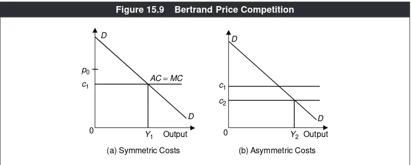
Look at Figure 15.9. The curve DDdepicts the market demand. For simplicity it is assumed that the marginal cost and the average cost are constant (independent of the output), that is, MC= AC.Panel (a) assumes that the average cost is same
AC = MC
c1
Y1
D p0
D
D
0 D
0
c2
Output Y2
(b) Asymmetric Costs c1
Output
(a) Symmetric Costs
for both firms, equal to c1. This is the symmetric cost case. Panel (b) depicts the asymmetric-cost case, where the average cost of firm B(= c2) is less than that of
firm A(=c!).
Let us begin with the symmetric-cost case. Suppose that any of the two firms, say firm A, charges a price higher than c1, say equal to p0. What is the optimal pric-ing strategy of firm B? There is no need to ‘calculate’ profits by weighing marginal revenue and marginal cost. The answer is ‘charge a price slightly less than p0‘. Why? It is because by doing so the firm Bwill capture the entire market. Of course, firm Acan recapture the entire market by charging a price slightly less than what firm Bis asking. This reasoning implies that the firms will continue to cut the price till no firm makes any abnormal profit. Thus, pA= pB= c1constitute the Nash equi-librium. Given pA= c1, firm Bhas no incentive to charge a higher price (thereby los-ing the entire market) or a lower price (thereby incurrlos-ing losses). Similarly, given
pB= c1, firm Ahas no incentive to change its price from pA= c1. In summary, when the product is homogeneous and average costs are the same across the firms, in Bertrand price competition, price = average cost is the Nash equilibrium. This implies that no firm makes any abnormal profits, that is, the profits are zero. Which firm sells how much? This is indeterminate. A natural assumption is that since the firms are symmetric, they will have equal shares in the market—each firm will have 50 per cent of the market, that is, sell 0Y1/2 in Figure 15.9(a). However, irre-spective of who sells how much, the total quantity sold is determined from the market demand curve at the price equal to the average cost—0Y1in Figure 15.9(a). It is noteworthy that under the same market and technology parameters, if the firms were competing in quantities, they would have made abnormal profits as in Cournot competition, the price is not driven down to the average cost. This yields a fundamental insight that price competition is more severe on the profits of firms in oligopoly than competition in quantity.
Consider now the asymmetric cost case. By the same logic, no price above c1can be in Nash equilibrium. But unlike the symmetric-cost case, pA =pB= c1do not
constitute the Nash equilibrium. It is because firm Bcan still charge a price lower than c1, drive firm Aout of the market and yet make a profit higher than that at
pB=c1. Hence, in Nash equilibrium, only the more efficient firm survives, and the
market price is the one, which is marginally lower than the average cost of the less efficient firm.
Indeed we can generalise the above conclusion to the case of many firms. Rank the firms starting from the most inefficient to the most efficient. Under price com-petition, only the most efficient firm survives because it can ‘under-cut’ in terms of price any other less efficient firm, thereby, driving all other firms out and capture the entire market.
NUMERICAL EXAMPLE 15.2
There are two companies, Gangajaaland Mahajaal, which supply bottled water to the twin cities of Bhubaneswar and Cuttack. In procuring, processing and pack-aging water bottles, each firm incurs a constant average cost of Rs 8 per bottle. The demand curve of bottled water in Bhubaneswar and Cuttack is given by the equa-tion Q=10,000 −250p. If the two firms play the Bertrand price competition game,
what will be market price and quantity sold?
This is a case of symmetric Bertrand competition. Hence the equilibrium price will be driven down the (common) average cost, that is, p=Rs 8. Substituting this
into the market demand function, the total quantity sold =Q=10,000 −250 ×8 =
10,000 −2,000 =8,000.
Whether Cournot or Bertrand?
Because quantity and price competition yield very different outcomes, one may ask which one is more appropriate. There is no single answer to this question. It depends on whether in the industry concerned, the firms commit to quantities they produce and let prices clear the market or commit to prices and let quantities clear the market. In producing steel, for instance, it is relatively time-consuming to change production levels (within say month or a quarter). Thus, steel firms have to commit to a production level and it is reasonable to assume quantity competition. But, in providing telephone service, for example, the prices (tariffs) are quoted in catalogues and on websites, which are not changed frequently; thus it is reasonable to assume price competition (that is, treat price as the strategic variable).
Cartel Issues
The Nash equilibrium in quantity or price competition is comparable to the Nash equilibrium in the Prisoner’s Dilemma game discussed in Chapter 13. Hence, essentially, oligopoly competition is a Prisoner’s Dilemma situation. It is because in oligopoly, the firms compete with one another rather than collude.
Colluding or collusion means jointly deciding the total output for the industry and the market price, and formulating an allocation rule as to who will produce how much. If the firms do collude, collectively they behave like a monopoly or a cartel. A cartel essentially raises the price of the product by restricting output. Under the cartel, the total (monopoly) profits are higher than the sum of the prof-its in oligopoly competition (irrespective of the form of oligopoly competition). The quota system dictating who produces how much is devised such that every member (firm) of the cartel is better off (that is, enjoys higher profit), compared to oligopoly competition.
there is no such concern because higher prices would hit the consumers in the foreign countries, not the domestic consumers. This is why, over time, many cartels have come up typically in international markets. OPEC is, of course, the best exam-ple. But cartels have been formed in many products including steel and vitamin.
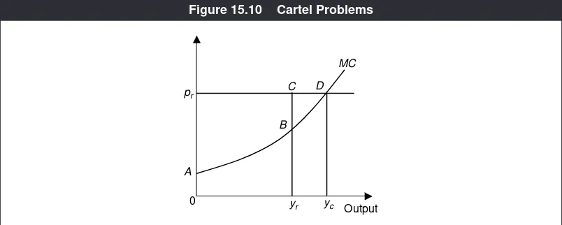
However, there is an inherent problem with any cartel, even if it may be legal—a member of a cartel has an incentive to ‘cheat’ and secretly break the already agreed upon cartel rules. This can be understood by using Figure 15.10.
The MCcurve denotes the marginal cost curve of a cartel member. Suppose the
cartel has fixed the price of the product at pr, which is presumably higher than the
price that would prevail under oligopoly competition. Such a high price is made sustainable by following a production (an export) quota rule in which each mem-ber is asked to produce a limited quantity (less than what it would have produced in oligopoly competition). Let this quantity or quota for the member in question
be yr. In the cartel regime, this member’s total revenues are thus equal to the area
0prCyr. Its total costs are measured by the area under the MCcurve, equal to the
area 0AByr. Hence, profits are equal to the area ABCpr.
Suppose this is the original situation—there is a cartel, in which the member
firms are charging the price pr,and each member is producing a limited quantity,
with yrbeing the output of a particular member firm. Now observe that as long as
the market price is given at pr, the particular firm we are looking at can actually
increase its output and sale up to yCand make higher profits because if the market
price is given, it is equal to MRand is over the output range 0 toyC, with MR>
MC. Indeed, at the output level yC, the firm’s profits will be equal to ADpr,which
is greater than ABCpr. The implication is that this member-firm will have an
incen-tive to break the cartel rules, over-produce and make greater profits.
Of course, once the ‘cheater’ sells more, there will be downward pressure on the market price. This will be ‘felt’ by the rest of the cartel members (who are ‘honest’ to the cartel) because they will face difficulty in selling their quota output at the
cartel price pr(since there is more quantity in the market than before—thanks to
yc pr
yr
MC
Output 0
B D
A
C
the cheater). Whether the cheater is identified or not, others will come to infer that someone among them has broken the rules. What happens next? A strong possibility is that the cartel is abandoned and the industry reverts to oligopoly competition.
In summary, insofar as the cheater is concerned, it gains in the short run and loses in the long run. If the firms value the future or trust each other very much, then no firm may decide to cheat in the first place. If not, cheating is an inherent problem, making the cartel inherently unstable. This is why, in the real world, it is hard to find an example of a cartel that has lasted successfully for a long stretch of time. Even OPEC has had its problems over years. The average cartel life (before it busts itself due to cheating and enforcement problems or gets busted by author-ities) is around four to six years.
ANTI-TRUST REGULATIONS
A common feature of almost any form of an imperfectly competitive market is that price exceeds marginal cost and, therefore, such a market entails a loss of social surplus. This is of concern especially from the viewpoint of consumers’ welfare. After all, the social purpose of businesses is to create/produce goods and services so as to meet our consumption needs and enhance our standard of living.
Thus, increasing concentration of firms (meaning smaller number of large size firms) in an industry is worrisome insofar as it results in higher prices for the con-sumers. This is indeed the basis of monopoly regulation, which we discussed in Chapter 14. It is also the rationale behind the so-called anti-trust regulationswith respect to oligopoly markets.
The origin of anti-trust regulations lies in the economic history of the US. During decades following the civil war in America, a selected group of aggressive entrepreneurs became extremely powerful, for example, Andrew Carnegie, Jay Gould, John Rockefeller and others. These men created huge empires of business for themselves and were accused of exploiting labour and using unfair labour practices. They were portrayed as ruthless businessmen who could do anything to increase their wealth and later came to be known as ‘robber barons’. Intense public sentiments led to the first major anti-trust law in the form of the Sherman Act of 1890. This marked the beginning of anti-trust regulation in the US and in the rest of the world. The initial aim of these regulations was to contain market concentration on the presumption that this is bad for the consumers for the rea-sons described above.
Anti-trust Practice in India
In India, the Monopoly and Restrictive Trade Practices (MRTP) Act of 1969 was the initiating legislation, whose aim was to restrict monopoly power. However, the MRTP interventions were nothing close to what is outlined above as the objective of a standard anti-trust legislation in a market oriented economy. They were mostly in the form of controls, licensing and permits. It was also largely ineffective, as both public-sector and private-sector monopolies thrived under it. Why? Because in terms of having real punitive powers, it was nearly toothless. To enforce its orders it had to depend on courts entirely, which would take years to reach any final decision. It did not have power to impose, on prima facie grounds, any initial penalties for breach of its directives, before the matter could be moved to the courts. It did not even have powers to enforce the attendance of a witness. The personnel at the disposal of MRTP did not have the right skills to deal with investigations of economic transactions.
Only very recently, India has passed the Competition Act in 2002, which has many innovative features. In effect, the MRTP Act has been repealed and the MRTP Commission dissolved. Following the Competition Act, a Competition Commission was set up in 2003. Its aim is to prevent ‘anti-competitive practices, promote and sustain competition, protect the interests of the consumers and ensure freedom of trade’ as the website of the Competition Commission states. Both goods and services sectors as well as private and public sector firms come under its purview. The Commission has the mandate to impose penalties initially
Clip 15.1: Microsoft’s Anti-trust Woes
on erring parties and provide relief to firms who are adversely affected by the anti-competitive strategies adopted by other firms. At the point of writing this book the Commission is in its formative stage, yet to initiate an anti-trust case.
Regulating the Telecom Sector
It is interesting that the telecom sector in India is oligopolistic, yet it is not subject to the ‘standard’ anti-trust regulations. Instead, there is a separate body called the Telecom Regulatory Authority of India, or briefly TRAI, established in 1997. Why is there a separate regulatory body for this industry only? It is because (i) this sec-tor provides a ‘basic’ utility, like telephony, which is unlike automobile or an inter-net browser and (ii) there are a few special features of this sector.
Because the industry offers a basic utility, TRAI regulates telecom prices, simi-lar to electricity regulatory commission fixing electricity tariffs. But there is much more. That is, the government recognises the vital role of the telecom sector in the growth and development of almost any other sector of the economy and, there-fore, its objective is to ensure a telecom sector that is world-class.
The technology of this sector is changing almost ‘day by day’, which is posing new problems and challenges. For instance, internet services are facilitating teleph-ony. Telephone and broadcasting industries are stepping into each other’s markets. The working difference between wireless lines and wired lines is getting narrowed. There is also an issue of ‘spectrum management’ or ‘frequency allocation’. As the demand for frequency is increasing dramatically, it must be used in an efficient manner, without interfering with those used by the national defence sector. Dealing with these complex issues and ensuring healthy competition in a vital sector like telecom are the reasons behind a separate regulatory body like TRAI.
Economic Facts and Insights
● In monopolistic competition, an individual firm, even though very small
compared to the entire market, has some market power because its product is differentiated. This implies that the firm is able to set a price above the marginal cost.
● Even though monopolistically competitive firms have market power, they
earn normal profits in the long run.
● Besides setting output and prices, firms in monopolistic competition and
oligopoly engage in advertising.
● There is no unified theory of oligopoly.
● An oligopoly market is characterised by game-theoretic, strategic interaction
among firms.
● Essentially, oligopoly competition yields a Prisoner’s Dilemma situation.
● The kinked demand curve model attempts to explain why in oligopoly
markets, prices may be relatively stable.
● Under quantity competition, an increase in the costs faced by one firm leads,
in equilibrium, to less output by this firm and more output by the rival firm.
● If the product is homogeneous and firms compete in prices, then the market
sustains only the most efficient firm(s).
● Price competition is more severe on the profits of firms in oligopoly than
competition in quantity.
● In a cartel where quantities to be produced by firms are restricted, that is,
each firm has a quote, an individual firm has an incentive to cheat in terms of producing and selling more than its quota. This implies that cartels are inherently unstable.
● The average life of a cartel in the international market is between four to six
years.
● The modern philosophy behind anti-trust laws and their enforcement is
that being big in business may not be necessarily bad. Central is the issue of whether merger and acquisitions or product/pricing strategies by big firms tend to serve the interests of consumers.
● In India the recently constituted Competition Commission is in charge of
anti-trust issues. The telecom sector, however, has a separate regulatory body, TRAI (Telecom Regulatory Authority of India).
E
E X
X E
E R
R C
C II S
S E
E S
S
15.1 Briefly explain the excess capacity theorem.
15.2 Suppose at a given point of time a monopolistically competitive firm faces the AR, MRand the cost curves as shown in Figure 15.1. (a) Is this a situation
of long-run equilibrium? (b) If not, will some new firms enter into or some existing firm exit from the industry?
15.3 The LACschedule of a representative firm under monopolistic competition,
is given as follows. In the long-run industry equilibrium, this firm produces an output, which is ____ than ____. Fill in the blanks and give reasons.
Output LAC
0 –
1 20
2 16
3 13
4 11
5 14
6 18