A Comprehensive Overview of Basic Clustering Algorithms

(1)

A Comprehensive Overview of Basic

Clustering Algorithms

Glenn Fung

(2)

1 Introduction

In recent years, the dramatic rise in the use of the web and the improve-ment in communications in general have transformed our society into one that strongly depends on information. The huge amount of data that is gen-erated by this communication process contains important information that accumulates daily in databases and is not easy to extract. The field of data mining developed as a means of extracting information and knowledge from databases to discover patterns or concepts that are not evident.

As stated in [24], machine learning provides the technical basis of data mining by extracting information from the raw data in the databases. The process usually consists of the following: transforming the data to a suitable format, cleaning it, and inferring or making conclusions regarding the data. Machine learning is divided into two primary sub-fields: supervised learn-ing and unsupervised learnlearn-ing. Within the category of unsupervised learnlearn-ing, one of the primary tools is clustering. This paper attempts to cover the main algorithms used for clustering, with a brief and simple description of each. For each algorithm, I have selected the most common version to represent the entire family. Advantages and drawbacks are commented for each case, and the general idea of possible sub-variations is presented.

In order to have a better understanding of the performance of different algorithms in practice, I compiled several representative implementations of various algorithms from the web. I chose the MATLAB[15] programming language for the implementation for two primary reasons. First, through my research, I have a significant amount of data available in that format and experience in using it. Second, due to the increasing popularity of this language, there is an extensive quantity of applications in this format.

In the conclusion, I use the theoretical survey and numerical results as the basis of recommendations for considerations to have in mind while choosing a specific method according to the properties of a given data set.

1.1 Supervised and Unsupervised Learning

(4)

be classified, the algorithm should predict a label for this case. Under this paradigm, there is the possibility of overfitting or “cheating” by memorizing all the labels for each case, rather than learning general predictive relation-ships between attribute values and labels. In order to avoid overfitting, these algorithms try to achieve a balance between fitting the training data and good generalization, this is usually referred as the Bias/Variance dilemma. The outcomes of this class of algorithms is usually evaluated on a disjoint set of examples from the training set, called the testing set. Methods range from traditional statistics approaches, neural networks and, lately, Support vector machines [5].

On the other hand, in unsupervised learning the algorithm is provided with just the data points and no labels, the task is to find a suitable rep-resentation of the underlying distribution of the data. One major approach to unsupervised learning is data clustering, which will be the focus of this paper.

Both supervised and unsupervised learning have been combined in what some people called semi-supervised learning [1],[8]. The unsupervised part is usually applied first to the data in order to make some assumptions about the distribution of the data, and then these assumptions are reinforced using a supervised approach.

2 What is Clustering?

A large number of clustering definitions can be found in the literature, from simple to elaborate. The simplest definition is shared among all and includes one fundamental concept: the grouping together of similar data items into clusters. A more elaborate definition, for example, is stated in [24], “These [obtained] clusters should reflect some mechanism at work in the domain from which instances or data points are drawn, a mechanism that causes some instances to bear a stronger resemblance to one another than they do to the remaining instances.” A simple, formal, mathematical definition of

clustering, as stated in [9] is the following: let X ∈Rm×n _{a set of data items}

representing a set of m points xi in Rn. The goal is to partition X into K

groups Ck such every data that belong to the same group are more “alike”

than data in different groups. Each of the K groups is called a cluster. The

result of the algorithm is an injective mapping X 7−→C of data items Xi to

(5)

The numberKmight be pre-assigned by the user or it can be an unknown,

determined by the algorithm. In this paper, I assume that the K is given by

the user.

The nature of the clustering problem is such that the ideal approach is equivalent to finding the global solution of a non-linear optimization problem. This is usually a difficult task to achieve. As a matter of fact, this is an np hard problem, e.g. a problem that can not be solved in polynomial time.

3 Applications of Clustering

Recently, clustering have been applied to a wide range of topics and areas. Uses of clustering techniques can be found in pattern recognition, as is the case of the paper: “Gaussian Mixture Models for Human Skin Color and its Applications in Image and Video databases” [25]; compression, as in “Vec-tor quantization by deterministic annealing”[13]; classification, as in “Semi-Supervised Support Vector Machines for Unlabeled Data Classification” [8]; and classic disciplines as psychology and business. This makes clustering a technique that merges and combines techniques from different disciplines such as mathematics, physics, math-programming, statistics, computer sci-ences, artificial intelligence and databases among others.

4 Background and notation

To make it easier for the reader understand the ideas behind the algorithms presented, I tried to “unify” the notation used in all of them. To achieve that, the following definitions are assumed in all of the algorithms:

• X ∈ Rm×n _{denotes a set of data items representing a set of} _m _points

xi in Rn

• Ck denoted the k-th cluster.

• K denotes the total number of clusters.

(6)

5 Clustering Methods

There are many different ways to express and formulate the clustering prob-lem, as a consequence, the obtained results and its interpretations depend strongly on the way the clustering problem was originally formulated. For example, the clusters or groups that are identified may be exclusive, so that every instance belongs in only one group. Or, they may be overlapping, meaning that one instance may fall into several clusters. Or they may be probabilistic, whereby an instance belongs to each group depending on a cer-tain assigned probability. Or they may be hierarchical, such that there is a crude division of the instances into groups at a high level that is further re-fined into a finer levels. Furthermore, different formulations lead to different algorithms to solve. If we also consider all the “variations” of each different algorithm proposed to solve each different formulation, we end up with a very large family of clustering algorithms. Although in the literature there are as many different classifications of clusterings algorithms as the number of algorithms itself, there is one simple classification that allows essentially splitting them into the following two main classes:

• Parametric Clustering

• Non-Parametric Clustering

5.1 Parametric Approaches

In general, parametric methods attempt to minimize a cost function or an optimality criterion which associates a cost to each instance-cluster assign-ment. The goal of this kind of algorithm is to solve an optimization problem to satisfy the optimality criterion imposed by the model, which is often means minimizing the cost function. This type of method usually includes some as-sumptions about the underlying data structure. This class of algorithms can be classified into two groups:

• Generative Models

• Reconstructive Models.

5.1.1 Generative Models or Probability-based Models

The basic idea of this kind of model is that the input vector or instances

(7)

Suppose the density of an observation xk with respect to Ei is given by

fi(xk|θ) for some unknown set of parameters θ. The probability that xk

be-longs to distributionEi is denoted byτki. Since usually each point is assumed

to belong to just one distribution, we have the constraint PK_i=1τi

k = 1. The

goal of the method is to find the parameters θ and τ that maximize the

likehood (or minimize the minus likehood):

L(θ, τ) =

Efficient iterative Expectation-Maximization (EM) schemes exist [7] to perform the optimization. The major problem with this model is that if the

parametersθ to be estimated are allowed to vary freely for each distribution,

then finding a global optimum for the problem can be be too time and space intensive for large problems. Usually, what is then found is a local minimum that depends strongly on the set of initial clusters that some algorithms of this kind require. A common criticism of these models (as of many others) is that they do not address the problem of “noise”in the data. A considerable number of papers trying to address this issue have been published in the last years.

These type of models also relies on the assumption that the data comes from a known distribution (usually Gaussian distribution) which can not be true in many cases; even worse the data may not be numerical, in which case this method can not be used. In particular, most databases contain a large amount of categorical data, where the notion of distance is not natural and has to be defined according to the case.

Generative mixture models, in contrast, offer several advantages due to the fact that they define a proper probability distribution in data space. Not only can they be used for conditional density estimation, but due to their probabilistic nature they also provide means for dealing with the problem of missing data and active data selection.

The following are representative examples of generative models.

5.1.2 The Gaussian Mixture model

In this approach, the data are viewed as coming from a mixture of probability Gaussian distributions, each representing a different cluster. As stated in

[7] the probability density function (p.d.f) of an observation x in the finite

(8)

p(x;θ) =

distributionEiandθdenotes the vector of all unknown parameters associated

with the parametric forms adopted for theseK component densities. For the

case of multivariate Gaussian components, θ consists of the elements of the

mean vectors µi, and the distinct elements of the covariance matrices Σi for

i= 1, . . . , K. The vector of unknowns (τ, θ) belongs to some parameter space and is estimated using the EM algorithm.

In this particular case of Gaussian components, the mixture density

con-tains the following adjustable parameters: τi,µi,and Σi (Σi is the covariance

matrix corresponding to the points in distribution Ei) for i= 1, . . . , K. The

negative log-likehood for the data set is given by

E=−lnL=−

which can be seen as an error function that will be minimized.

(9)

where,

3. calculate the change in the error function:

∆t+1 ₌_Et+1₋_Et₌₋

5.1.3 C-Means Fuzzy Clustering

Instead of determining whether or not an event occurs, as is the case with probability, fuzziness measures the degree to which an event occurs. Ac-cording to proponents of fuzziness, fuzzy probability allows the traditional notion of probability to be extended. As a consequence, different aspects of the human experience can be more effectively characterized. Whether or not fuzziness or probability models the physical process found in nature more effectively depends exclusively on the specific process and, in general, is unknown.

The goal of traditional clustering is to assign each data point to one and only one cluster. In contrast, fuzzy clustering assigns different degrees of membership to each point. The membership of a point is thus shared among various clusters. This creates the concept of fuzzy boundaries which differs from the traditional concept of well-defined boundaries.

Bezdek [2] asserts that the well-defined boundary model usually does not reflect the description of real data. This assertion led him to develop a new family of clustering algorithms based on a fuzzy extension of the least-square error criterion.

Typical of parametric approaches, this algorithm attempts to minimize a cost-function and a local minimizer is attained, instead of a global. In

this case the following cost-function is minimized, with respect toU , a fuzzy

K-partition of the data set, and toC, a set ofK prototypes (cluster centers):

(10)

whereqis any real number greater than 1,Xjis thejth n-dimensional feature

vector, Ci is the centroid of the ith cluster, uij is the degree of membership

of Xj in the ith cluster, d2(Xj, Ci) is any inner product metric (distance

between xj and Ci) M is the number of data points, K is the number of

clusters. The parameter q is the weighting exponent foruij and controls the

“fuzziness” of the resulting clusters.

The algorithm below is based on finding a “good” fuzzy partition of the data, which is carried out through an iterative optimization of (2).

Algorithm 5.2 Fuzzy C-means Clustering Algorithm 1. Choose primary centroids Ci (prototypes)

2. Compute the degree of membership of all feature vectors in all the clus-ters:

and update the memberships, uij to uˆij according to step 2.

4. if maxijkuij −uˆijk< tol stop, otherwise goto step 3.

It is important to note that the computation of the degree of membership

uij depends on the definition of the distance measure d2(Xj, Ck).

5.1.4 Reconstructive Models

As mentioned above, reconstructive methods generally attempt to minimize a cost function. The essential difference in the various types of reconstruc-tive algorithms lies in the techniques used to model and minimize the cost function. One of the most basic, straightforward clustering techniques is the

(11)

father of this entire family of algorithms. K-means forms clusters in numeric

domains, partitioning instances into disjoint clusters. Variations of K-means

where the Euclidean distance function is replaced by another distance have been proposed. It has been shown that the performance of the method is strongly related to the distance used [3].

Although this algorithm is easy to implement, it has the drawback of being greedy in the sense that it tends to get stuck in a local minimum that usually depends on the initial center provided. This makes this algorithm very sensitive to initial points. As an alternative to the problem of local min-imum, stochastic methods with a close relation to physics, such as variations of simulated annealing [21], have been applied to clustering optimization problems.

Instead of assigning the points to the closest center in the regional space, the points can be mapped to a higher dimensional space, related to the regional data space, by a nonlinear mapping. There is no need to compute the mapping explicitly, instead it can be computed via a certain kernel function that relates the inner products from the original space to the inner products in the higher dimensional space. This idea led to a family of algorithms called topographic clustering algorithms [14].

5.1.5 K-means and K-median

The K-means algorithm, probably the first one of the clustering algorithms

proposed, is based on a very simple idea: Given a set of initial clusters, assign each point to one of them, then each cluster center is replaced by the mean point on the respective cluster. These two simple steps are repeated until convergence. A point is assigned to the cluster which is close in Euclidean distance to the point.

AlthoughK-means has the great advantage of being easy to implement,

it has two big drawbacks. First, it can be really slow since in each step the distance between each point to each cluster has to be calculated, which can be really expensive in the presence of a large dataset. Second, this method is really sensitive to the provided initial clusters, however, in recent years , this problem has been addressed with some degree of success [23].

If instead of the Euclidean distance the 1-norm distance is used:

d(x, y) =

n

X

i=1

(12)

a variation of K-means is obtained and it is called K-median, in [3] the authors claim that this variation is less sensitive to outliers than traditional

K-means due to the characteristics of the 1-norm.

Both algorithms are presented below.

Algorithm 5.3 k-Means (Median) Algorithm Given C₁j, . . . , C_kj at it-eration j, compute C₁j+1, . . . , C_kj+1 by the following two steps:

(a) Cluster Assignment: For each H′

i, i = 1, . . . t, determine ℓ(i) such

that C_ℓ(i)j is closest to H′

i in the Euclidean (one) norm.

(b) Cluster Center Update: For ℓ = 1, . . . , k choose C_ℓj+1 as a mean (median) of all H′

i assigned to C j ℓ.

Stop when C_ℓj+1 =C_ℓj.

5.1.6 Deterministic annealing

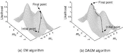
The Simulating Annealing (SA) method was developed by Kirkpatrick et al [21] in analogy to an experimental annealing procedure, where the stability of metal or glass is improved by heating or cooling. Solutions for an op-timization problem are heated and heated in simulations to find a “good” quality solution, i.e. one admissible solution with very low cost. In the case of clustering, a solution which achieved a low value of the associated cost function can be accepted. While convergence in probability to the global minimum has been established, SA techniques are often slow because of its randomized stochastic search in the whole parameter space. Deterministic Annealing (DA) methods intend to overcome this deficiency, while preserving the main advantages of SA [21]. SA estimates relevant expectation values of the system parameters reducing the search space by optimizing over a probabilistic admissible state space of the parameters, instead of the whole space.

(13)

Figure 1: In the estimation of two parameters m₁_, m₂ _{the EM goes to a local}

minimum while DAEM reaches the global minimum

As shown in Figure 2, by gradually decreasing the temperature until F exactly agrees with the likelihood function and minimizing the free energy at each temperature, the global optimal solution can be obtained. Note that unlike the conventional simulated annealing (SA), the free energy is deterministically minimized t each temperature. Therefore the DA is much faster than the SA [12].

Figure 2: Annealing control by the temperature The optimization at each

(14)

Due to the complexity of the algorithm and the notation needed, the actual algorithm is not presented here but it can found in [12].

5.2 Non-Parametric Approaches

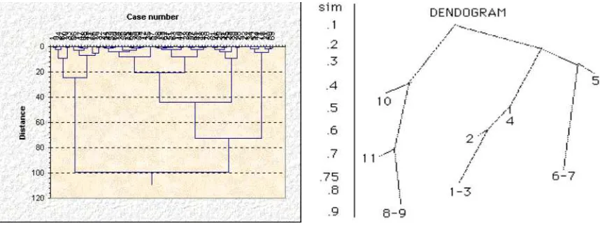
Two good representative examples of the non-parametric approach to clus-tering are the agglomerative and divisive algorithms, also called hierarchical algorithms, that produce dendograms. Both methods are based in the mea-sures of the dissimilarities among the current cluster set in each iteration. Agglomerative algorithms merge some of the clusters, depending on how sim-ilar they are, and divisive algorithm splits them. In this section, I will focus on the agglomerative algorithm, but all these ideas apply to the divisive al-gorithm as well. A dendogram is simply a tree that shows which cluster were agglomerated in each step. It can be easily broken at selected links to obtain cluster or groups of desired cardinality or radius. This number of cluster or groups can also be determined as a function of some merging threshold. The idea is that with a threshold of zero, the number of clusters is equal of the number of data points, and with a high threshold the data is partitioned in just one single cluster. Since the dendogram is just a tree, its structure representation is also easy to generate and to store. The major drawback of this kind of approach is that the entire dendogram is sensitive to previous (and possible erroneous) cluster merging i.e data are not permitted to change cluster membership once assignment has taken place [6]. An important ad-vantage of non-parametric clustering methods is that they do not make any assumptions about the underlying data distribution. Furthermore, they do not require a explicit representation of the data in a Euclidean form. they only require a matrix with the pairwise similarities based on a predefined distance. However such a matrix containing the pairwise similarities

some-times can require a lot of storage space, usually of the order o(m2_{), where}

m is the number of data points to be clustered, thus making the algorithm

(15)

Figure 3: Example of dendograms

5.2.1 The Hierarchical Clustering Algorithms

A representative algorithm of this kind is hierarchical clustering, which is implemented in the popular numerical software MATLAB [15]. This algo-rithm is an agglomerative algoalgo-rithm that has several variations depending on the metric used to measure the distances among the clusters. The Euclidean distance is usually used for individual points . There are no known criteria of which clustering distance should be used, and it seems to depend strongly on the dataset. Among the most used variations of the hierarchical clustering based on different distance measures are [19]:

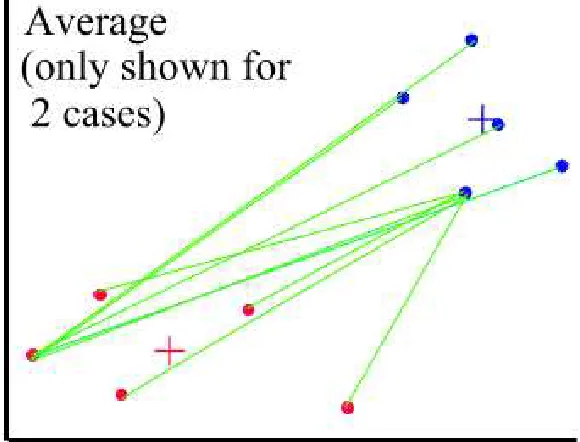
1. Average linkage clustering

The dissimilarity between clusters is calculated using average values. The average distance is calculated from the distance between each point in a cluster and all other points in another cluster. The two clusters with the lowest average distance are joined together to form the new cluster.

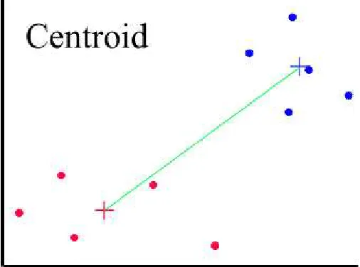
2. Centroid linkage clustering

(16)

Figure 4: Average linkage clustering

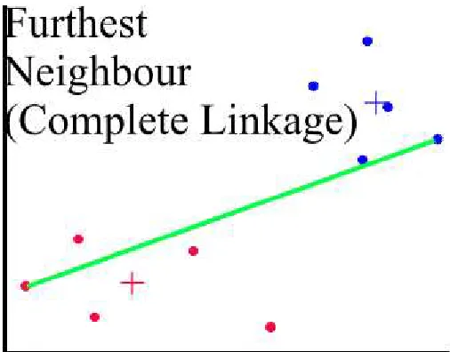
3. Complete linkage clustering (Maximum or Furthest-Neighbor Method) The dissimilarity between 2 groups is equal to the greatest dissimilarity between a member of cluster i and a member of cluster j. This method tends to produce very tight clusters of similar cases.

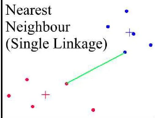
4. Single linkage clustering (Minimum or Nearest-Neighbor Method): The dissimilarity between 2 clusters is the minimum dissimilarity between members of the two clusters. This method produces long chains which form loose, straggly clusters.

5. Ward’s Method: Cluster membership is assigned by calculating the to-tal sum of squared deviations from the mean of a cluster. The criterion for fusion is that it should produce the smallest possible increase in the error sum of squares.

In all the graphics, the red and blue + signs mark the centers of the two clusters and the points are represented by red and blue dots.

(17)

Figure 5: Centroid linkage clustering

Algorithm 5.4 Single linkage clustering algorithm Let be D(i, j) the distance between clusters i ,in this case defined as was describe above, and j and N(i) the nearest neighbor of cluster i.

1. Initialize as many clusters as data points

2. For each pair of clusters (i, j) compute D(i, j)

3. For each cluster i compute N(i)

4. Repeat until obtain the desired number of clusters

(a) Determine i, j such that D(i, j) is minimized (b) Agglomerate cluster i and j

(c) Update each D(i, j) and N(i) as necessary

(18)

Figure 6: Complete linkage clustering (Maximum or Furthest-Neighbor Method)

6 Numerical Tests

All our computations were performed on the University of Wisconsin Data Mining Institute “locop1” machine, which utilizes a 400 Mhz Pentium II and allows a maximum of 2 Gigabytes of memory for each process. This computer runs on Windows NT server 4.0, with MATLAB 6 installed. Even though “locop1” is a multiprocessor machine, only one processor was used for all the experiments since MATLAB is a single threaded application and does not distribute any load across processors [15].

All the results, including time and number of iterations, for all the possible combinations of pairs (method, initial clusters) are reported in tables 1 to 4. For the checkerboard, figures 8 to 19, show a graphical representation of the dataset, the initial clusters and the obtained final cluster centers.

Another uncertain issue related to clustering is how to measure the per-formance of a given algorithm, for simplicity I chose one of the suggested

in [3], that they call Training set correctness, which is measured by the

(19)

Figure 7: Single linkage clustering (Minimum or Nearest-Neighbor Method)

the performance of the clustering algorithms.

6.1 The Algorithms tested

Due to the popularity of MATLAB, a wide range of applications can be found coded using this language. I did an extensive web search trying to find some clustering implementation to test on. After, selection I ended up with four of them:

1. An implementation of theK-means algorithm (kmeans.m):

This implementation is a variation of the k-median algorithm that was

done by a former UW computer Sciences department student, Paul Bradley, and it was used for the calculations in [3]. if the initial clusters are not provided, it will calculate them , using the bins idea, that will be described further on. This code can be found in /afs/cs.wisc.edu/

u/g/f/gfung/public/k median. The inputs for this algorithms are:

a matrix whose rows are the data points to be clustered, number of

clusters to be found K, and initials clusters as an optional input.

(20)

(the trial version) from the mathworks website: www.mathworks.com/ products/fuzzylogic/tryit.shtml. No initial clusters are needed since the algorithm calculates an initial fuzzy partition matrix from the given data. The required inputs are: a matrix whose rows are the data points

to be clustered ,number of clusters to be foundK, and an optional

vec-tor containing variations of the stopping criteria.

3. An implementation of A Gaussian Mixture model (gmm.m): This pro-gram was written by Roger Jang in Tsing Hua University in Taiwan and can be found in http://neural.cs.nthu.edu.tw/jang/matlab/demo/. The required inputs are: a matrix whose rows are the data points to

be clustered, number of clusters to be found K, and an optional vector

containing variations of the stopping criteria. this code is a small vari-ation to the original Gaussian Mixture cluster, the difference consists in a heuristic that is applied to perturb the clusters centers whenever one of them does not capture a “fair share” of the data.

4. An implementation of single link hierarchical clustering (clusterdata.m) This program is part of the MATLAB statistic toolbox which is part of the MATLAB version used in the computer sciences Lab. The required inputs are: a matrix whose rows are the data points to be clustered,

number of clusters to be foundK. Also the user can choose the distance

between cluster to be used. This distance can be any of the variations described in section 5.2.1.

It important to clarify that the results shown in this paper, depends on the effectiveness the implementation of each algorithm, this numbers can vary significantly when tested with different versions of the same algorithm. The main purpose of this experiments is to provide the reader with an rough idea of the general behavior of each method tested.

6.2 About the Initial points

In order to have a sense of the local behavior of each algorithm, different sets of initial cluster were used (in the algorithms were it was required as an input). The different methods to calculate the initial set of clusters were:

1. Corner: Since all the values in the data sets were scaled to be in

(21)

consider. This is usually a “bad” set of initial points since it lies on the boundary of the data, and can be considered an outlier.

2. Bins: This method consists in divide the space in bins and then take

random points inside each bin, this assure that the set of initial points are distributed covering the entire dataset.

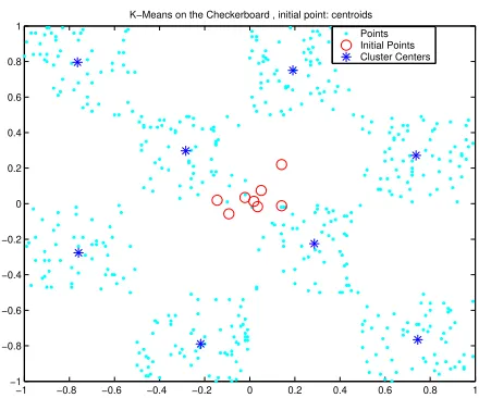
3. Centroid: This method consists in chose all the starting clusters close to the mass centroid of the dataset. Each cluster center is calculated adding a small random perturbation to the centroid of the dataset.

4. Spread: The cluster centers are distributing randomly and trying to cover the entire space. This method is similar to bins.

5. PCA: The data points are projected in the space of the principal

com-ponent, then a clustering procedure is applied to this one-dimensional set. The cluster centers are calculated then, depending of the obtained

clusters in the one-dimensional space. In this paper I applied the K

-means algorithm to the obtained projected lower dimensional data.

6.3 Datasets used in the testing

Most of the algorithms tested have versions to handle categorical data, but in such cases a good similarity or distance function has to be provided. Finding a good similarity function depends strongly on the dataset and it is not an easy task to define a “good” one. For simplicity the numerical test were performed in dataset which attributes are numerical values. The four chosen datasets are often used for testing and referred on the literature. All the

values in the datasets were normalized to have values in [−1,1].

The numerical experiments performed in each dataset are divided in sev-eral sections and are shown next.

6.3.1 Results on the Checkerboard Dataset

(22)

the methods work, and also to give an idea of the performance of the different algorithms, starting from different cluster centers.

−1 −0.8 −0.6 −0.4 −0.2 0 0.2 0.4 0.6 0.8 1 −1

−0.8 −0.6 −0.4 −0.2 0 0.2 0.4 0.6 0.8 1

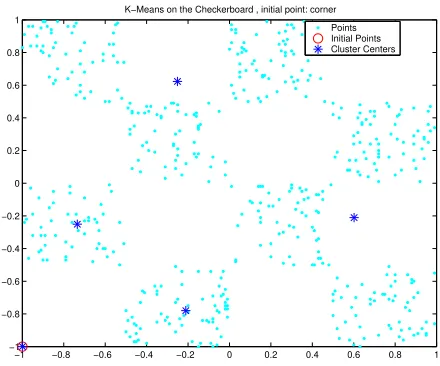
K−Means on the Checkerboard , initial point: corner Points Initial Points Cluster Centers

Figure 8: The K_{-means algorithm applied to the checkerboard dataset, initial}

(23)

−1 −0.8 −0.6 −0.4 −0.2 0 0.2 0.4 0.6 0.8 1

K−Means on the Checkerboard , initial point: bins Points Initial Points Cluster Centers

Figure 9: The K_{-means algorithm applied to the checkerboard dataset, initial}

clusters are calculated using the bin heuristic. A good final set of cluster centers is obtained.

K−Means on the Checkerboard , initial point: centroids Points Initial Points Cluster Centers

Figure 10: TheK_{-means algorithm applied to the checkerboard dataset, initial}

(24)

−1 −0.8 −0.6 −0.4 −0.2 0 0.2 0.4 0.6 0.8 1

K−Means on the Checkerboard , initial point: spread Points Initial Points Cluster Centers

clusters are calculated by spreading initial cluster centers among the whole data space.A medium quality set of final clusters is obtained.

−1 −0.8 −0.6 −0.4 −0.2 0 0.2 0.4 0.6 0.8 1

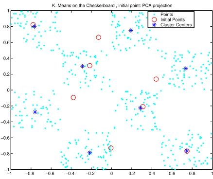
K−Means on the Checkerboard , initial point: PCA projection Points Initial Points Cluster Centers

(25)

−1 −0.8 −0.6 −0.4 −0.2 0 0.2 0.4 0.6 0.8 1

C−Means Fuzzy logic algorithm on the checkerboard, no initial points required Points Cluster Centers

Figure 13: The C_{-means Fuzzy clustering algorithm applied to the}

checker-board dataset, initial clusters are not required by this algorithm. A good final set of cluster centers is obtained.

−1 −0.8 −0.6 −0.4 −0.2 0 0.2 0.4 0.6 0.8 1

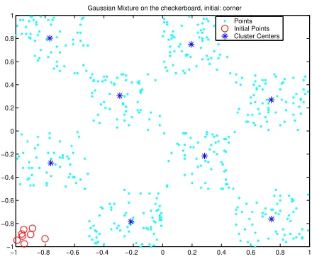
Gaussian Mixture on the checkerboard, initial: corner Points Initial Points Cluster Centers

Figure 14: The Gaussian Mixture algorithm applied to the checkerboard

(26)

−1 −0.8 −0.6 −0.4 −0.2 0 0.2 0.4 0.6 0.8 1

Gaussian Mixture on the checkerboard, initial: bins Points Initial Points Cluster Centers

dataset, initial clusters are calculated using the bin heuristic. A good final set of cluster centers is obtained.

−1 −0.8 −0.6 −0.4 −0.2 0 0.2 0.4 0.6 0.8 1

Gaussian Mixture on the checkerboard, initial: centroid Points Initial Points Cluster Centers

Figure 16: Gaussian Mixture algorithm applied to the checkerboard dataset,

(27)

−1 −0.8 −0.6 −0.4 −0.2 0 0.2 0.4 0.6 0.8 1

Gaussian Mixture on the checkerboard, initial: spread Points Initial Points Cluster Centers

dataset, initial clusters are calculated using spreading initial cluster centers among the whole data space. A good final set of cluster centers is obtained.

−1 −0.8 −0.6 −0.4 −0.2 0 0.2 0.4 0.6 0.8 1

Gaussian Mixture on the checkerboard, initial: PCA projection Points Initial Points Cluster Centers

(28)

−1 −0.8 −0.6 −0.4 −0.2 0 0.2 0.4 0.6 0.8 1

Hierarchical clustering on the checkerboard, no initial points required Points Initial Points Cluster Centers

Figure 19: The single linkage algorithm applied to the checkerboard dataset,

initial clusters are not required by the algorithm. A medium quality set of cluster centers is obtained.

The obtained results are summarized in table 1.

6.3.2 Results on the Galaxy Dim dataset

The Galaxy Dim dataset was used first in galaxy discrimination with neural networks in [18]. This dataset consists of 4192 instances and 14 attributes all of them real-valued continuous. There are two classes that are relatively easy to identify in this dataset. The classes classify galaxies according to their light content. Supervised approaches achieved accuracy of about 94% training correctness on this dataset. The obtained results are summarized on the table 2.

6.3.3 Results on the Wisconsin Breast Cancer Prognosis Dataset

(29)

Table 1: Comparisons of performance of K -Means,C-Means Fuzzy, Gaussian Mixture and Single-Link for the checkerboard dataset, correctness percentages and times are reported.

Method K-Means C-M. Fuzzy Gaussian Mix. S-Link

Initial point Correct. % Correct. % Correct. % Correct. % Time (Sec.) Time (Sec.) Time (Sec.) Time (Sec.)

Corner 52.26 98.76∗

99.38 76.13∗

3.06 0.45∗

1.84 9.59∗

Bins 99.79 - 99.38

-1.17 - 0.48

-Centroid 99.79 - 99.38

-2.79 - 2.78

-Spread 87.44 - 99.38

-2.34 - 0.67

-PCA 99.38 - 99.38

(30)

-Table 2: Comparisons of performance of K -Means,C-Means Fuzzy, Gaussian Mixture and Single-Link for the Galaxy Dim dataset, correctness percentages and times are reported.

Corner 50.33 85.01∗

85.97 Out Of Mem.

2.03 1.43 ∗

4.70

-Bins 84.49 - 86.42

-14.95 - 0.26

-Centroid 84.49 - 85.97

-16.89 - 1.26

-Spread 84.49 - 85.97

-14.90 - 1.42

-PCA 32.32 - 25.88

(31)

-Table 3: Comparisons of performance of K -Means,C-Means Fuzzy, Gaussian Mixture and Single-Link for the WBCP dataset, correctness percentages and times are reported.

Method _K-Means C-M. Fuzzy Gaussian Mix. S-Link

Corner 62.74 92.44 92.44 63.09

0.32 0.42 0.21 18.51

Bins 92.09 - 92.44

-0.75 - 0.20

-Centroid 92.09 - 0.07

-1.34 - 88.75

-Spread 92.09 - 0.07

-1.48 - 88.92

-PCA 17.92 - 62.74

-11.12 - 31.68

-correctness on this dataset, meaning that the two groups are relatively easy to identify. The obtained results are summarized on the table 3.

6.3.4 Results on Census dataset

The Census dataset is a version of the US Census Bureau “Adult” dataset, which is publicly available from Silicon Graphics website [4]. The dataset contains 20,000 instances and 10 numeric attributes. The data can be clas-sified in two groups dividing people according it economic status based on the indicators contained in the 10 given attributes. Supervised approaches achieved accuracy of about 94% training correctness on this dataset. Results are summarized on table 4.

6.4 General comments on the obtained results

(32)

Table 4: Comparisons of performance of K -Means,C-Means Fuzzy, Gaussian Mixture and Single-Link for the Census dataset, correctness percentages and times are reported.

Corner 64.52 81.61 81.66 Out of Mem.

9.48 4.29 17.95

-Bins 81.7 - 81.66

-37.84 - 2.17

-Centroid 81.70 - 81.65

-33.18 - 2.93

-Spread 81.70 - 81.32

-38.03 - 1.09

-PCA 43.62 - 80.89

(33)

-• As was expected theK-means algorithm was strongly sensitive to initial points, the quality of the obtained final clusters depended strongly on the given initial set of clusters. Bins and centroid provided the best initials clusters for this algorithm. This algorithm was generally, the second slower one.

• The worst performance was obtained from the single-link hierarchical

clustering algorithm. In two cases it fails due to memory constrains when tried to store the entire matrix of similarities of points. Even in the small datasets the final cluster obtained were of poor-medium quality compared to the obtained by the other algorithms. Although this is an implementation included in a official MATLAB toobox, I think the poor performance is based in a poor quality implementation of this algorithm.

• The C-Means algorithm performed really well, in all four datasets the

correctness obtained was comparable to the best ones achieved. this algorithm was not the faster but it was not the slower either, so the performance speed was acceptable.

• The Gaussian Mixture Model was in general the fastest and the more

robust one. It gave good final clusters starting from almost all the initial points tested. With the exception of the case where PCA was used to get the initial clusters, this algorithm performed obtained really good performance and was the faster one.

• An interesting thing to notice is that the PCA technique gives really

(34)

7 Conclusions and Future Directions

Given a data set, the ideal scenario would be to have a given set of criteria to choose a proper clustering algorithm to apply. Choosing a clustering algo-rithm, however, can be a difficult task. Even finding just the most relevant approaches for a given data set is hard. Most of the algorithms generally assume some implicit structure in the data set. The problem, however, is that usually you have little or no information regarding the structure, which is, paradoxically, what you want to uncover.

The worst case would be one in which previous information about the data or the clusters is unknown, and a process of trial and error is the best option. However, there are many elements that are usually known, and can be helpful in choosing an algorithm. One of the most important elements is the nature of the data and the nature of the desired cluster. Another issue to keep in mind is the kind of input and tools that the algorithm requires. For example, some algorithms use numerical inputs, some use categorical inputs; some require a definition of a distance or similarity measures for the data. The size of the data set is also important to keep in mind, because most of the clustering algorithms require multiple data scans to achieve convergence, a good discussion of this problems and its relation to databases can be found in “Scaling Clustering Algorithms to Large Databases” by Usama Fayyad et al.[20]. Recently, new scalable clustering frameworks have been developed. Some examples are BIRCH [22], CLARANS [17].

An additional issue related to selecting an algorithm is correctly choosing the initial set of clusters. As was shown in the numerical results, an adequate choice of clusters can strongly influence both the quality of and the time re-quired to obtain a solution. Also important is that some clustering methods, such as hierarchical clustering, need a distance matrix which contains all the distances between every pair of elements in the data set. While these

methods rely on simplicity, the size of this matrix is of the size m2_{, which}

can be prohibitive due to memory constraints, as was shown in the experi-ments. Recently this issue has been addressed, resulting in new variations of hierarchical and reciprocal nearest neighbor clustering.

(35)

References

[1] K. P. Bennett and A. Demiriz. Semi-supervised support vector machines.

In M. S. Kearns, S. A. Solla, and D. A. Cohn, editors,Advances in Neural

Information Processing Systems -10-, pages 368–374, Cambridge, MA, 1998. MIT Press.

[2] J. C. Bezdek. Pattern Recognition with Fuzzy Objective Function

Algo-rithms. New York, 1981.

[3] P. S. Bradley, O. L. Mangasarian, and W. N. Street. Clustering via concave minimization. In M. C. Mozer, M. I. Jordan, and T. Petsche,

editors, Advances in Neural Information Processing Systems -9-, pages

368–374, Cambridge, MA, 1997. MIT Press. ftp://ftp.cs.wisc.edu/math-prog/tech-reports/96-03.ps.

[4] US Census Bureau. Adult dataset. Publicly available from:

www.sgi.com/Technology/mlc/db/.

[5] C. J. C. Burges. A tutorial on support vector machines for pattern

recognition. Data Mining and Knowledge Discovery, 2(2):121–167, 1998.

[6] D. fasulo. An analisys of recent work on clustering algortihms. Technical report, 1999.

[7] C. fraley and E. Raftery. How many clusters? which clustering method?, answers via model-based cluster analisys. Technical Report 329, Dept. of Stattistics. University of Washington, Seattle, 1998.

[8] G. Fung and O. L. Mangasarian. Semi-supervised support vector

ma-chines for unlabeled data classification. Optimization Methods and

Soft-ware, 15(1), April 2001.

ftp://ftp.cs.wisc.edu/pub/dmi/tech-reports/99-05.ps.

[9] T. Graepel. Statistical physics of clustering algortihms. Technical Re-port 171822, FB Physik, Institut fur Theoretische Physic, 1998.

[10] T. K. Ho and E. M. Kleinberg. Building projectable classifiers

of arbitrary complexity. In Proceedings of the 13th International

(36)

1996. http://cm.bell-labs.com/who/tkh/pubs.html. Checker dataset at: ftp://ftp.cs.wisc.edu/math-prog/cpo-dataset/machine-learn/checker.

[11] T. K. Ho and E. M. Kleinberg. Checkerboard dataset, 1996.

http://www.cs.wisc.edu/math-prog/mpml.html.

[12] T. Hofmann and J. Buhmann. Pairwise data clustering by determinis-tic annealing. Technical report, Institut fur Informatik III, Rheinische Friedrich-Wilhelms-Universitat, bonn, 1996.

[13] E. Gurewitz K. Rose and G. C. Fox. Vector quantization by deterministic annealing.

[14] J. MacQueen. Some methods for classification and analysis of

multi-variate observations. California, 1967.

[15] MATLAB. User’s Guide. The

Math-Works, Inc., Natick, MA 01760, 1994-2001.

http://www.mathworks.com/access/helpdesk/help/techdoc/matlab.shtml.

[16] P. M. Murphy and D. W. Aha. UCI repository of machine learning

databases, 1992. www.ics.uci.edu/∼mlearn/MLRepository.html.

[17] R. Ng and J. Han. Efficient and effective clustering methods for spatial

data mining. In VLDB-94, 1994.

[18] S. Odewahn, E. Stockwell, R. Pennington, R. Hummphreys, and W.

Zu-mach. Automated star/galaxy discrimination with neural networks.

As-tronomical Journal, 103(1):318–331, 1992.

[19] C. Olson. Parallel algorithms for hierarchical clustering.

[20] U. Fayyad P. Bradley and C. Reina. Scaling clustering algorithms to large databases. Technical Report MSR-TR-98-37, Microsoft, Redmon, WA, 1998.

[21] C. Gelatt S. Kirkpatrick and M. Vecchi. Optimization by simulated annealing. 220:671–680, 1983.

[22] R. Ramakrishnan T. Zhang and M. Livny. Birch: a new data

clus-tering algorithm and its applications. In Data Mining and Knowlegde

(37)

[23] C. Reina U.M. Fayyad and P.S. Bradley. Initialization of iterative re-finement clustering algorithms.

[24] I. Witten and E. Frank. Data Mining.

A Comprehensive Overview of Basic Clustering Algorithms