Contents lists available atScienceDirect
Pattern Recognition
journal homepage:w w w . e l s e v i e r . c o m / l o c a t e / p r
A multi-prototype clustering algorithm
Manhua Liu
a,∗, Xudong Jiang
b, Alex C. Kot
baDepartment of Instrument Science and Engineering, Shanghai Jiao Tong University, No. 800, Dong Chuan Road, Shanghai, 200240, PR China bEEE, Nanyang Technological University, 50 Nanyang Avenue, Singapore 639798, Singapore
A R T I C L E I N F O A B S T R A C T
Article history:
Received 21 November 2006 Received in revised form 28 May 2008 Accepted 9 September 2008 Keywords:
Data clustering Cluster prototype Separation measure Squared-error clustering
Clustering is an important unsupervised learning technique widely used to discover the inherent structure of a given data set. Some existing clustering algorithms uses single prototype to represent each cluster, which may not adequately model the clusters of arbitrary shape and size and hence limit the clustering performance on complex data structure. This paper proposes a clustering algorithm to represent one cluster by multiple prototypes. The squared-error clustering is used to produce a number of prototypes to locate the regions of high density because of its low computational cost and yet good performance. A sep-aration measure is proposed to evaluate how well two prototypes are separated. Multiple prototypes with small separations are grouped into a given number of clusters in the agglomerative method. New proto-types are iteratively added to improve the poor cluster separations. As a result, the proposed algorithm can discover the clusters of complex structure with robustness to initial settings. Experimental results on both synthetic and real data sets demonstrate the effectiveness of the proposed clustering algorithm.
© 2008 Elsevier Ltd. All rights reserved.
1. Introduction
Clustering is the unsupervised classification of patterns into groups[1]. It is widely used in data analysis such as data mining, pattern recognition and information retrieval. The Voronoi diagram also provides a means of naturally partitioning space into subre-gions to facilitate spatial data analysis and has been applied for data clustering[2–5]. But this technique often implies emphasis on the shape and arrangement of patterns, i.e., the geometric aspect of groups. Clustering techniques have been widely studied in Refs. [6–19]. They suggest more on grouping behavior and can be broadly classified into hierarchical or partitional clustering[1].
Hierarchical clustering is a procedure of transforming the prox-imity matrix of the data set into a sequence of nested groups in an agglomerative or divisive manner. The agglomerative hierarchi-cal clustering has been widely studied as it allows for more feasible segments to be investigated[7–11]. TheSingle-link[7],Complete-link
[8]andaverage-link[7]algorithms produce a sequence of clusterings based on the rank order of proximities. TheSingle-linkand Complete-linkalgorithms use the distance between two closest and farthest points of two clusters as the cluster distance, respectively. Depen-dence on a few data points to measure the cluster distance makes
∗Corresponding author. Department of Instrument Science and Engineering, School of Electronic, Information and Electrical Engineering, Shanghai Jiao Tong Uni-versity, No. 800, Dong Chuan Road, Shanghai 200240, China. Tel.: +86 34205206; fax: +86 34201372.
E-mail address:[email protected](M. Liu).
0031-3203/$ - see front matter©2008 Elsevier Ltd. All rights reserved. doi:10.1016/j.patcog.2008.09.015
these algorithms sensitive to noise. The average-link algorithm is more robust to noise by using the average distance of all pairs of patterns from different clusters as the cluster distance. A CURE algo-rithm[9]represents each cluster with a certain fixed number of well scattered points and shrinks these points toward the cluster center by a specified fraction. This algorithm achieves an improvement of noise robustness over theSingle-linkalgorithm. A Chameleon algo-rithm[10]partitions a constructed k-nearest neighbor graph into a number of subclusters followed by dynamically merging the subclus-ters. In general, the hierarchical clustering algorithms can provide an easy understanding of the inherent structure of the data set. But they often require high computational cost and large memory space which make them inefficient for large data sets.
sides the squared error, other criterions such as the Davies–Bouldin index[32]and cluster variance are imposed as a global criterion to determine the optimum number of clusters[26,31]. Most partitional clustering algorithms require less memory space and computation cost than the hierarchical clustering algorithms. But their cluster-ing results are usually not as good as those of hierarchical clus-tering. Recently, support vector clustering is proposed to generate the cluster boundaries of arbitrary shape by transforming the orig-inal space to a high dimensional space with a kernel function[19]. Although this algorithm can solve some difficult clustering problems, it is not easy to choose a suitable kernel parameter and the cluster-ing result cannot provide information about the representation of cluster.
The hybrid clustering algorithms are proposed to combine the merits of partitional and hierarchical clustering algorithms for bet-ter data grouping[12–15,33,34]. They usually partition the data set into a relatively large number of small subclusters and construct a hierarchical structure for them based on a certain cluster distance (similarity) measure. A given number of clusters can be found on the hierarchical structure. A BIRCH algorithm[12]arranges the data set into a number of subclusters represented bycluster feature(CF) vectors in a tree structure. It is efficient for large data sets.
In some applications, we may need to efficiently represent data and reduce the data complexity through clustering. A single pro-totype for each cluster, e.g., the centroid or medoid of cluster in K-means type clustering, may not adequately model the clusters of arbitrary shape and size and hence limit the clustering performance on the complex data structure. This paper proposes a clustering algorithm to represent a cluster by multiple prototypes. The re-maining of this paper is organized as follows. Section 2 reviews the related work along with the discussion of their differences. Section 3 presents the proposed multi-prototype clustering algorithm. In Section 4, the proposed algorithm is tested on both synthetic and real data sets and the results are compared to some existing clus-tering algorithms. Section 5 gives the conclusions.
2. Related work
The squared-error clustering algorithm produces a partition of the data set which aims to minimize the squared error[1,25,30]. LetX= {X1,X2, . . . ,XN}whereXi=[xi,1,xi,2, . . . ,xi,M]∈
R
Mbe a set ofNpatterns represented as points inM-dimensional space andK be the number of clusters. The cluster prototypes are denoted by a set of vectorsZ= {Z1,Z2, . . . ,ZK}. The squared error function is of clusterland Euclidean distance measure is often used.K-means clustering algorithm is a simple squared-error clustering algorithm with the number of clusters prespecified [25,27]. The processing steps of theK-means clustering algorithm can be summarized asZq
Zl
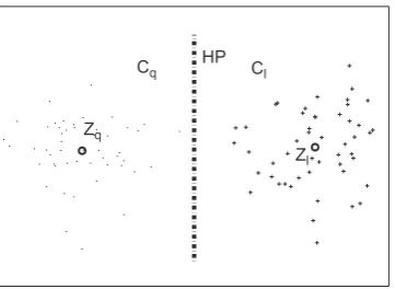
Fig. 1.The separating hyperplane of clusterCqandClrepresented by prototypeZq
andZl, respectively, in squared-error clustering.
follows[1]:
(1) Randomly chooseKcluster prototypes.
(2) For each pattern, compute its distances to all prototypes and assign it to the closest cluster as
ui,l=
(3) Update the prototype of each cluster as
Zl=
(4) Go to step (2) until convergence is achieved.
The K-means clustering algorithm has been widely used in data partitioning because of its low computation and memory space re-quirements and yet good performance in finding the regions of high density. But the result is sensitive to the initial partition. ISODATA (iterative self-organizing data analysis techniques) algorithm alle-viates this problem by iteratively deleting small clusters, merging similar clusters and splitting large clusters until a desired partition is obtained[30]. However, ISODATA algorithm uses single prototype (i.e., centroid) to represent each cluster, which may not adequately model the clusters of arbitrary shape and size no matter how well the data set is partitioned. In the squared-error clustering, the sep-arating boundary for each pair of clusters is the hyperplane through the midpoint of the cluster prototypes and perpendicular to the line connecting these prototypes (see Fig. 1). It may reside in the re-gion of high density for complex clusters (e.g., the separating hyper-planes for two clusters of different size inFig. 2a and arbitrary shape inFig. 2c). The hybrid algorithm[13]begins withK-means cluster-ing to partition the data set into a set of subclusters and apply the
Single-linkalgorithm to merge them into a given number of clusters according to their cohesions. More complex boundary can be con-structed to separate the clusters. But the boundary may still reside in the high-density region resulting in poor cluster separation when the initial partition ofK-means clustering is not properly set.
Z1
Z2 Z2 Z3 Z1
Z1 Z2
Z1 Z2
Z4 Z8
Z3 Z5
Z6 Z7
Z9
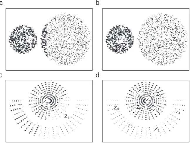
Fig. 2.Clustered data represented by different marks and prototypes denoted by text `Zl': (a) poor result with two clusters of different size modelled by `Z1' and `Z2', (b) good result with the small cluster modelled by `Z2' and the large cluster modelled by `Z1' and `Z3', (c) poor result with two clusters of arbitrary shape modelled by `Z1' and `Z2' and (d) good result with one cluster modelled by `Z1,Z2,Z4,Z8' and another cluster modelled by `Z3,Z5,Z6,Z7,Z9'.
others is that we propose a new cluster separation criterion and our algorithm is targeted at improving the cluster separation.
3. The proposed clustering algorithm
In this section, we first propose a separation measure to evalu-ate how well two cluster prototypes are separevalu-ated. Next, we present the proposed multi-prototype clustering algorithm based on the sep-aration measure. Finally, the complexity analysis of the proposed algorithm is provided.
3.1. Separation measure
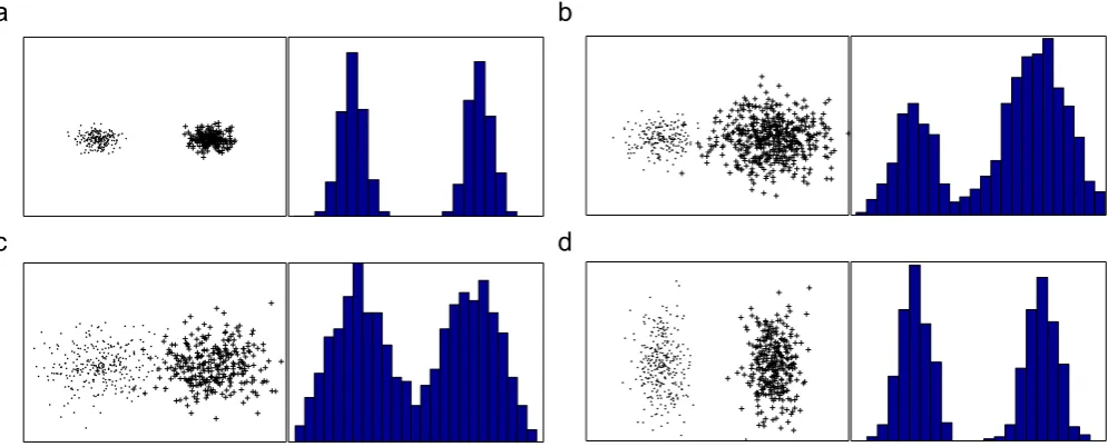
The separation of two clusters measures how well the clusters are separated. Conceptually, large separation of two clusters indi-cates less inclination of integrating these clusters into a larger one. It is also called cluster distance or similarity in the literature[7–10]. The distances between the closest or farthest data points of two clusters are used to measure the cluster separation in the agglom-erative clustering algorithms[7,8]. They are not only computation expensive but also sensitive to noise due to the dependence on a few points. In the prototype-based clustering algorithms, the sepa-ration of two clusters (or prototypes) is often measured using the distance between their prototypes. Although this measure is compu-tationally efficient and robust to noise, it cannot distinguish the clus-ters of different sizes and shapes. For example, four pairs of clusclus-ters inFig. 3have equal prototype distances, but their separations are obviously different. A measure of within-to-between cluster spread Rq,l=(e(Zq)+e(Zl))/d(Zq,Zl), wheree(Zl) is the within-cluster vari-ance andd(Zq,Zl) is the distance between the prototypeZq andZl, is introduced to evaluate the cluster separation[32]. Including the information of within-cluster variance solves the problem of cluster size but leave the cluster shape problem unsolved. For example, the Rof two clusters inFig. 3d is 0.2931 which is larger than that in Fig. 3c, 0.2455. But two clusters inFig. 3d are obviously better sep-arated than those inFig. 3c. A similarity measure of two clusters is
proposed by assuming the data distribution of each cluster follows a static model[13]. Although this measure is effective in some cases, it may not adapt to the internal characteristics of the clusters espe-cially when the data set contains the clusters of diverse shapes and distributions.
The cluster prototypes produced by the squared-error clustering are often located in the high-density region. Two prototypes con-nected by a region of high density are more likely to belong to one cluster than those connected by a sparse region. We propose a sep-aration measure based on the data distribution between two cluster prototypes to evaluate how well the prototypes are separated by a sparse region. Firstly, two cluster prototypes are connected by a line segment.The data points of two clusters are projected onto the line connecting the prototypes since the separating hyperplane is per-pendicular to it. LetZqandZldenote the prototypes of clusterCqand Cl, respectively. The projections of the data points are computed by
x′=(X−m0) T(Z
q−Zl) Zq−Zl2 , X∈C
q∪Cl, (5)
wherem0=(Zq+Zl)/2 is corresponding to the origin of the projections x′. Two cluster prototypes are projected at the positions−1
2 and12 of the line.
Fig. 3.Four pairs of clusters and their 1-D projected distributions. Their separations are: (a)sp=1 (b)sp=0.8219 (c)sp=0.6372 and (d)sp=0.9930.
on these data densities until only one local minimum exists on them.
Finally, the separation is computed based on the projected data distribution between the prototypes. If the minimum of the 2B+1 densities between two prototypes is large, the prototypes are con-nected by a relatively high-density region and hence are inclined to belong to one cluster. Based on the minimum density normalized by the average of those at two prototypes, the separation is computed by
spq,l=1−
2 min2B+1k=1 f −1 2+
k−1 2B
f −1 2
+f 1 2
. (6)
Largespq,lindicates that clusterClandCqor their prototypes are well separated by a sparse region. Some examples of the separa-tions between two clusters are shown inFig. 3. Instead of assuming a static distribution model, the data distribution is automatically es-timated in this separation measure which can adapt to the internal characteristics of individual clusters.
The separation in Eq. (6) is based on the minimum data density so that the separating boundary is assumed at the hyperplane through the most sparse region between two prototypes. However, two clus-ters are separated by the hyperplane through the midpoint of the prototypes in practice. By replacing the minimum density with the density at the midpoint of two prototypes in Eq. (6), we compute the separation of two prototypes based on the current separating hyperplane as
sp0q,l=1− 2f(0)
f(−12)+f(12). (7)
Ifsp0
q,l is small, the separating hyperplane resides in the high-density region between two prototypes. Obviously,sp0q,l
spq,l.3.2. The proposed multi-prototype clustering algorithm
For a given data set, the natural clusters often exist in the con-tinuous regions of relatively high density separated by the sparse areas in the pattern space. Using single prototype to represent each cluster often result in the cluster boundaries residing in the region of high density (seeFig. 2a and c). By adding one or more prototypes
to model the clusters, the cluster boundary can move to the sparse region of the pattern space (seeFig. 2b) or a more complex boundary can be constructed to separate the complex clusters (seeFig. 2d). We propose a clustering algorithm in which multiple prototypes coexist-ing within a continuous region of relatively high density are grouped to model the cluster and new prototypes are iteratively added to improve the poor cluster boundaries.
Firstly, we partition the data set into a relatively large number of small subclusters with each one represented by a prototype. Let P (K
P < N) be the number of prototypes for theK clusters. The squared-error clustering has good performance in finding the regions of high density with high computational efficiency and low mem-ory space. It is thus employed in this stage to producePprototypes. However, thePprototypes may not be appropriately distributed in the high-density regions. Some prototypes may represent the large subclusters consisting of the patterns belonging to different clusters and form a connection between two natural clusters. In addition, some prototypes may reside in the outliers which do not belong to any cluster. Thus, we try to add prototypes in the large subclusters and remove the noise prototypes. For each subclusterl, we com-pute the within-cluster squared errorEland the number of patterns Nl. The large subcluster usually has both largeNlandElwhile the noise subcluster often has small Nl. We remove the noise proto-types withNl< Nmin(Nmin=0.3N/Pin our experiments) and add a new prototype in the large subcluster withNl>2.5NminandEl> Emax (Emax=Pk=1Ek/P+
std(Ek),>0). The squared-error clustering isrepeated until no prototypes are added or removed.
Next, multiple prototypes coexisting within a continuous region of relatively high density are grouped to model the cluster based on the separation measure in Eq. (6). We compute the separationspq,l between each pair of prototypes and form a separation matrix of P×P. Ifspq,lis small, prototypeqandlcoexist in a high-density region and can be grouped into one cluster. The separation of two multi-prototype clustersCmandCnis defined as the smallest separation of two prototypes from different clusters
cspm,n= min
Zl∈Cm,Zq∈Cnspl,q. (8)
organized to representKclusters in the agglomerative method. Thus, the separating boundary of two clusters is composed of multiple hyperplanes determined by the pairs of prototypes from different clusters. For example, the separating boundary of two clusters in Fig. 2d is composed of five hyperplanes determined by the pairs of prototypes: {Z7,Z8},{Z9,Z8},{Z9,Z2},{Z6,Z1},{Z6,Z4} and{Z5,Z4}. By grouping multiple prototypes to represent a cluster, complex boundaries can be obtained to separate the non-linearly separable clusters.
The last step is to improve the poor cluster boundaries. The cluster boundary may not reside in the sparse region between two clusters due to the poor initial settings. Adding new prototype can push the poor cluster boundary move to the sparse region or con-struct a more complex boundary to separate the clusters. Thesp0q,lin Eq. (7) is used to check the separation of cluster hyperplane. If sp0q,l< T, the cluster separating hyperplane is poor. We computesp0q,l for each pair of prototypes from different clusters and sort the poor ones (sp0
q,l< T) in increasing order. For each pair of prototypes sorted bysp0q,l, ifNq+Nl>3Nminand the separating boundary of the clusters the prototypes belong to has no new prototype already been added to, a new prototype is added to improve the poor cluster boundary. The new prototype is computed as the mean vector of the patterns whose projectionsx′locate in [−1
4,14].
After adding new prototypes, the multi-prototype clustering al-gorithm repeats the above steps until the prototypes do not change. Each pattern in the data set belongs to the cluster consisting of the closest prototype. The processing steps of the proposed algorithm can be summarized as:
(1) Initially setP
Kand randomly choosePcluster prototypes from the data set.(2) Apply the squared-error clustering on the data set to obtainP subclusters with each one represented by a prototype. (3) Remove the prototypes of subclusters withNl< Nmin and
de-creasePaccordingly. Add a new prototype in the large subclus-ters withNl>2.5NminandEl> Emaxand increasePaccordingly. If there are prototypes removed or added, go to step (2). (4) Calculate the separationsspq,lbetween each pair of prototypes
and produce a separation matrix.
(5) Organize thePprototypes intoKclusters based on the separation matrix. Two clusters with the smallest separation are iteratively grouped into one cluster untilKclusters are obtained.
(6) Compute the separationsp0q,lbetween each pair of prototypes
from different clusters and sort the poor ones (sp0
q,l< T) in in-creasing order.
(7) For each pair of prototypes sorted bysp0q,l, ifNq+Nl>3Nmin and the separating boundary of the clusters the prototypes be-long to has no new prototype already been added to, add a new prototype between these two prototypes and increaseP accord-ingly. The new prototype is computed as the mean vector of the patterns whose projectionsx′locate in[−1
4,14]. (8) Go to step (2) until the prototypes do not change. (9) Output the clustering result.
3.3. Complexity analysis
Letmbe the number of iterations in the squared-error clustering. The time complexity isO(NPm) for partitioning the data set to pro-duceP prototypes. It isO(P2logP) for the prototype organization which is similar to theSingle-link algorithm. Thus, the time com-plexity of the proposed clustering algorithm isO(NPm+P2logP). The space complexity is O(N) for the partitioning of the data set in the squared-error clustering. In the prototype organization, the
space complexity isO(P2) because a separation matrix of sizeP×P has to be stored. Thus, the space complexity of the proposed clus-tering algorithm isO(N+P2). The number of prototypesPis much smaller thanN. Thus, the proposed clustering algorithm requires less memory space and computation cost than the commonly used hier-archical clustering algorithms such asSingle-linkandComplete-link
while preserves much of the speed and efficiency of the squared-error clustering algorithm.
4. Experimental results and comparisons
The proposed multi-prototype clustering algorithm can be ap-plied for any numerical data set. We conduct a series of experiments on both synthetic and real data sets to demonstrate the clustering performance of the proposed algorithm. The results are compared to some existing clustering algorithms.
4.1. Synthetic data
Clusters on two-dimensional (2D) data sets are easy to visualize and compare. This section tests the proposed clustering algorithm on five synthetic 2D data sets. For good visualization of the clustering re-sults, we represent the clustered data by different marks and denote the prototypes with texts (For example, `Zl' denotes prototypel).
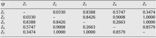
To illustrate the process of the proposed algorithm, we first con-sider the data set shown inFig. 2c which consists of two clusters of arbitrary shape and size. The clustering result withP=K(K=2) is shown inFig. 2c.K prototypes cannot adequately model the clus-ters. Our clustering algorithm initializesPas 5 and setTto 0.8. Since only two clusters exist in the data set, a new prototype is added in each iteration.Fig. 4a shows an initial clustering state of five proto-types produced by the squared-error clustering. The separationspq,l between each pair of the five prototypes is computed andTable 1 shows the separation matrix. In cluster organization, prototypeZ1 andZ2with the smallest separation are first grouped into one cluster {Z1,Z2}. The second smallest separation issp3,4so thatZ3andZ4are organized into another cluster{Z3,Z4}. The left prototypeZ1are orga-nized into the same cluster asZ5i.e.{Z1,Z2,Z5}sincesp1,5is the third smallest separation. The cluster boundary is composed of the hyper-planes separating four pairs of prototypes, {Z3,Z2},{Z3,Z1},{Z4,Z1} and{Z4,Z5}. We compute thesp0
q,lbetween these pairs of prototypes. A new prototype is added betweenZ1andZ4since thesp01,4=0.4253 is the smallest among them. If the above steps are repeated, an in-termediate clustering state of eight prototypes is obtained as shown inFig. 4b. Since the smallest separationsp0
q,lbetween two clusters is sp04,5=0.7460< T, a new prototype is added betweenZ4andZ5. The clustering algorithm terminates atP=10 when the smallest separa-tion between two clusterssp04,10=0.8400> T.Fig. 4c shows the final clustering result of 10 prototypes. We can see that two clusters are correctly discovered.
In addition, we apply the proposed algorithm on four 2D data sets which are often used to test the clustering algorithms[9,10,12,13,22]. Fig. 5shows the four 2D data sets denoted as DB1, DB2, DB3 and DB4, respectively. DB1 is obtained from Ref.[9]. It contains one big and two small circles and two ellipsoids connected by a chain of
Table 1
The separation matrix of five prototypes inFig. 4a
sp Z1 Z2 Z3 Z4 Z5
Z1 – 0.0330 0.8388 0.5747 0.3474
Z2 0.0330 – 0.8426 0.9008 1.0000
Z3 0.8388 0.8426 – 0.2663 1.0000
Z4 0.5747 0.9008 0.2663 – 0.8579
Z1
Z2 Z5
Z3 Z4
Z1
Z4
Z2 Z8
Z3 Z5
Z6 Z7
Z1
Z4
Z2 Z8
Z3 Z5
Z6 Z7
Z10 Z9
Fig. 4.An illustrative example of our clustering algorithm where `◦` denotes the new added prototype: (a) initial clustering state of five prototypes, (b) an intermediate clustering state of eight prototypes and (c) final clustering result of 10 prototypes.
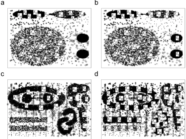
Fig. 5.Four 2D data sets used in our experiments: (a) DB1 with 8000 data points, (b) DB2 with 8000 data points, (c) DB3 with 10,000 data points and (d) DB4 with 8000 data points.
outliers. The other three data sets DB2, DB3 and DB4 are obtained from[10]. These data sets with 8000 to 10,000 data points consist of the clusters of arbitrary shape and size and the outliers are scattered on the data sets, which represent some difficult clustering instances. Fig. 6shows the clustering results of the proposed algorithm on these 2D data sets. The total number of prototypes finally obtained to model the clusters are 11, 29, 38 and 59 for the DB1, DB2, DB3 and DB4, respectively. From these figures, we can see that the proposed algorithm successfully discovers the clusters on these data sets.
Fig. 6.The clustering results of our proposed algorithm on the four 2D data sets: (a) DB1 with 11 prototypes, (b) DB2 with 29 prototypes, (c) DB3 with 38 prototypes and (d) DB4 with 59 prototypes.
Fig. 7.The clustering results of the proposed algorithm on poor initialization (a) the initial partition of DB1; (b) final result of 21 prototypes on DB1; (c) the initial partition of DB3 and (d) final result of 47 prototypes on DB3.
initial prototypes also result in poor clustering result where two small circles on the right are modelled into one cluster by a pro-totype. Our proposed algorithm iteratively adds new prototypes to improve the poor cluster boundaries resulted by the inappropriate initial settings.Fig. 7b and d show the final clustering results of 21 prototypes on DB1 and 47 prototypes on DB3, respectively. We can see the clusters on these data sets are successfully discovered.
We compare the proposed algorithm with some existing cluster-ing algorithms on the four 2D data sets. As these data sets contain
theSingle-linkequipped with outlier elimination, DBScan and CURE algorithms can correctly discover the clusters on one or two of the first three data sets but all fail on the complex DB4. The hybrid al-gorithm[13] is able to discover the clusters of the four data sets. However, its clustering result is sensitive to the initial settings. As reported in Ref.[13], the probabilities of successful partitions are about 95%, 90%, 65% and 40% on the DB1, DB2, DB3 and DB4, respec-tively, after performing this hybrid algorithm 20 times with random initialization on each data set. Similarly, the proposed algorithm is performed on each of the four 2D data sets over 20 random runs with the initial number of prototypes set to 3K. The probabilities of the successful partitions are 100%, 100%, 95% and 90% on the DB1, DB2, DB3 and DB4, respectively. The average numbers of prototypes to finally model the clusters are 17, 26, 39 and 62 for DB1, DB2, DB3 and DB4, respectively. Thus, more prototypes are usually required to represent the clusters which are more complex in shape and size.
4.2. Real data
To show the practical applicability of our proposed multi-prototype clustering algorithm, we apply it on three real data sets: Iris data, Wine Recognition Data and Wisconsin Breast Cancer (WBC) Data, which are available at UCI Machine Learning Repository[35]. The class label is given for each pattern in these data sets. It is ignored during the clustering but used for evaluation of clustering performance. In this work, the clustering error rate is used to evalu-ate the performance of clustering algorithm. It is computed by[27]:
Error=the number of misclassified patterns
the number of patterns in data set ×100%. (9)
To compute the clustering error rate, the major problem is the correspondence between the given class labels and the found clus-ters. We perform the matching between them. A clusterlcorresponds to class labelqif the number of patterns labelled asqinlis larger than those of other class labels. The best matching of the clusters is selected as the correspondence to the class labels.
We compare our proposed algorithm with some existing clus-tering algorithms such asK-means, agglomerative hierarchical clus-tering and hybrid algorithms on these real data sets. The proposed algorithm is performed on each data set over 20 random runs and the best clustering result is presented. We implement theK-means algorithm with a good initialization of the cluster centers in Ref.[27] on the WBC Data while the clustering results on the other two real data sets are reported in Ref.[27]. We perform the three common ag-glomerative clustering algorithms:Single-link[7],Complete-link[8] andAverage-link[7]on each data set and present the best cluster-ing result of them. In addition, the hybrid algorithm[13]is also im-plemented on these real data sets with our best effort. We give the best clustering result after 20 random runs of it on each data set. For other clustering algorithms, we present the results reported in the literature.
The Iris data set consists of 150 patterns and each one is repre-sented by four numerical features: sepal length, sepal width, petal length and petal width. Three types of Iris flowers: setosa, versi-color and virginica are labelled as class I, II and III, respectively. Each class consists of 50 patterns. This data set is often used to test the clustering algorithms and the clustering results of three clusters are reported in Refs.[15,27]. Ref.[15]also gives the clustering re-sults by theSingle-linkandComplete-linkalgorithms. Our algorithm produces five prototypes to model the three clusters on this data set. One prototype is used to represent cluster C1 which is easier to be
algorithm link
C1 50 0 0 2.67 11.33 4.0 4.0 7.4
C2 0 47 1
C3 0 3 49
Table 3
The clustering results for Wine Recognition data
Found cluster Given class Clustering error rate (%) I (59) II (71) III (48) Our
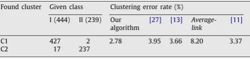
The clustering results for Wisconsin Breast Cancer data Found cluster Given class Clustering error rate (%)
I (444) II (239) Our
separated from others. Two prototypes are used to represent each of cluster C2 and C3.Table 2summarizes the clustering results for this real data set. We can see our algorithm performs better than other clustering algorithms.
The Wine Recognition data set contains the results of a chemical analysis of the wines grown in the same region in Italy but derived from three different cultivars. The wines from three cultivars repre-sent three types of wine data labelled as class I, II and III, respectively. This data set consists of 178 patterns and each one is represented by 13 features such as alcohol, magnesium, color intensity, etc. The feature values are normalized to [0, 1] to balance the effects of the features measured on different scales. This data set is also used to test the clustering algorithm[23,27]. Five prototypes are produced in our algorithm to model the three clusters on this data set. Two prototypes are used to represent each of cluster C1 and C2. Cluster C3 is represented by one prototype.Table 3shows the clustering re-sults for this real data set. We can see that the clustering result of our algorithm is better than those of others.
The WBC data set consists of 683 patterns which belong to two types of patterns: 444 benigns and 239 malignants labelled as class I and II, respectively. Each pattern is represented by nine features. This data set is also used to test the clustering algorithm[11]. As stated in Ref.[11], its clustering result is better than those in Refs.[17,18]. Our algorithm produces four prototypes to model the two clusters on this data set. One prototype is used to represent cluster C1 and the other three prototypes represent cluster C2. The clustering results for this real data set are shown inTable 4. Our algorithm performs better than other clustering algorithms on this data set.
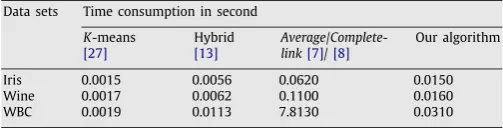
Table 5
The comparison of computational complexity on the three data sets Data sets Time consumption in second
K-means
with theK-means and hybrid[13] algorithms due to the iteration of adding new prototypes. To alleviate this problem, we can ini-tially set more prototypes in the squared-error clustering so that fewer prototypes will be added afterwards. In addition, we can con-sider re-clustering the data of the clusters affected by new proto-types instead of the whole data set to reduce the computation cost. Table 5shows the computation time of our algorithm compared with theK-means, hierarchical and hybrid clustering algorithms on the three real data sets. All the algorithms are implemented in MATLAB and executed on a Dell Precision PWS390 1.86 GHz PC with 1 GB memory running Windows XP professional. Although our algorithm requires a little more computation than theK-means and hybrid [13] algorithms, it is much faster than the hierarchical clustering algorithms.
5. Conclusions
In this paper, we have proposed a multi-prototype clustering al-gorithm which can discover the clusters of arbitrary shape and size. The squared-error clustering is used to produce a number of pro-totypes and locate the regions of high density because of its low computation and memory space requirements and yet good perfor-mance. A separation measure is proposed to evaluate how well two prototypes are separated by a sparse region. Multiple prototypes with small separations are organized to model a given number of clusters in the agglomerative method. New prototypes are iteratively added to improve the poor cluster boundaries resulted by the poor initial settings. The proposed algorithm requires less memory space and computation cost than the commonly used hierarchical cluster-ing algorithms such asSingle-linkandComplete-linkwhile preserves much of the speed and efficiency of the squared-error clustering al-gorithm. Experimental results on both synthetic and real data sets show the effectiveness of the proposed clustering algorithm.
References
[1] A.K. Jain, R.C. Dubes, Algorithms for Clustering Data, Prentice-Hall, Englewood Cliffs, NJ, 1988.
[2] A. Okabe, B. Boots, K. Sugihara, S.N. Chui, Spatial Tessellations, Concepts and Applications of Voronoi Diagrams, Wiley, New York, 2000.
[3] H. Koivistoinen, M. Ruuska, T. Elomaa, A Voronoi diagram approach to autonomous clustering, discovery science, Proceedings of the 9th International Conference, Springer, Berlin, 2006, pp. 149–160.
[4] C. Reyes, M. Adjouadi, A clustering technique for random data classification, IEEE International Conference on Systems, Man and Cybernetics, vol.1, October 1995, pp. 316–321.
[5] J. Li, P. Hao, Hierarchical structuring of data on manifolds, IEEE Conference on Computer Vision and Pattern Recognition, June 2007, pp. 1–8.
[6] A.K. Jain, M. Murthy, P. Flynn, Data clustering: a review, ACM Comput. Surveys 31 (3) (1999) 264–323.
[7] P.H.A. Sneath, R.R. Sokal, Numerical Taxonomy, Freeman, San Francisco, London, 1973.
[8] B. King, Step-wise clustering procedures, J. Am. Statist. Assoc. 69 (1967) 86–101.
[9] S. Guha, R. Rastogi, K. Shim, Cure: an efficient clustering algorithm for large databases, Proceedings of the Conference on Management of Data (ACM SIGMOD), 1998, pp. 73–84.
[10] G. Karypis, E.-H.S. Han, V. Kumar, Chameleon: a hierarchical clustering algorithm using dynamic modeling, IEEE Comput. 32 (8) (1999) 68–75.
[11] A.L. Fred, J.M. Leitao, A new cluster isolation criterion based on dissimilarity increments, IEEE Trans. Pattern Anal. Mach. Intell. 25 (8) (2003) 944–958. [12] T. Zhang, R. Ramakrishnan, M. Livny, Birch: an efficient data clustering method
for very large databases, Proceedings of the Conference on Management of Data (ACM SIGMOD), 1996, pp. 103–114.
[13] C.-R. Lin, M.-S. Chen, Combining partitional and hierarchical algorithms for robust and efficient data clustering with cohesion self-merging, IEEE Trans. Knowl. Data Eng. 17 (2) (2005) 145–159.
[14] M.N. Murty, G. Krishan, A hybrid clustering procedure for concentric and chain-like clusters, Int. J. Comput. Inform. Sci. 10 (6) (1981) 397–412.
[15] E.Y. Cheu, Z.Z. Chee Keong Kwoh, On the two-level hybrid clustering algorithm, The International Conference on Artificial Intelligence in Science and Technology (AISAT), 2004, pp. 138–142.
[16] A. Topchy, A.K. Jain, W. Punch, Clustering ensembles: models of consensus and weak partitions, IEEE Trans. Pattern Anal. Mach. Intell. 27 (12) (2005) 1866–1881.
[17] R. Kothari, D. Pitts, On finding the number of clusters, Pattern Recognition Lett. 20 (1999) 405–416.
[18] S.V. Chakravarthy, J. Ghosh, Scale-based clustering using the radial basis function network, IEEE Trans. Neural Networks 7 (1996) 1250–1261.
[19] A. Ben-Hur, D. Horn, H.T. Siegelmann, V. Vapnik, Support vector clustering, J. Mach. Learn. Res. (2) (2001) 125–137.
[20] G. McLachlan K. Basford, Mixture Models: Inference and Application to Clustering, Marcel Dekker, New York, 1988.
[21] M. Figueiredo, A. Jain, Unsupervised learning of finite mixture models, IEEE Trans. Pattern Anal. Mach. Intell. 24 (3) (2002) 381–396.
[22] M. Ester, H.-P. Kriegel, J. Sander, X. Xu, A density-based algorithm for discovering clusters in large spatial databases with noise, Proceedings of the 2nd International Conference on Knowledge Discovery and Data Mining (KDD), 1996, pp. 226–231.
[23] Y. Shi, Y. Song, A. Zhang, A shrinking-based clustering approach for multidimensional data, IEEE Trans. Knowl. Data Eng. 17 (10) (2005) 1389–1403. [24] M. Ankerst M.M. Breunig H.-P. Kriegel, J. Sander, Optics: ordering points to identify the clustering structure, Proceedings of the ACM SIGMOD International Conference on Management of Data (SIGMOD), 1999, pp. 49–60.
[25] J. McQueen, Some methods for classification and analysis of multivariate observations, Fifth Berkeley Symposium on Mathematical Statistics and Probability 1 (1967) 281–297.
[26] M. Sarkar, B. Yegnanarayana, D. Khemani, A clustering algorithm using an evolutionary programming-based approach, Pattern Recognition Lett. 18 (1997) 975–986.
[27] S.S. Khan, A. Ahmad, Cluster center initialization algorithm for k-means clustering, Pattern Recognition Lett. 25 (2004) 1293–1302.
[28] M.-C. Su, C.-H. Chou, A modified version of the k-means algorithm with a distance based on cluster symmetry, IEEE Trans. Pattern Anal. Mach. Intell. 23 (6) (2001) 674–680.
[29] D. Charalampidis, A modified k-means algorithm for circular invariant clustering, IEEE Trans. Pattern Anal. Mach. Intell. 27 (12) (2005) 1856–1865. [30] G.H. Ball, D.J. Hall, Isodata, a novel method of data analysis and classification,
Technique Report, Stanford University, 1965.
[31] C.J. Veenman, M.J. Reinders, E. Backer, A maximum variance clustering algorithm, IEEE Trans. Pattern Anal. Mach. Intell. 24 (9) (2002) 1273–1280. [32] D. Davies, D. Bouldin, A cluster separation measure, IEEE Trans. Pattern Anal.
Mach. Intell. 1 (4) (1979) 224–227.
[33] E.W. Tyree, J.A. Long, The use of linked line segments for cluster representation and data reduction, Pattern Recognition Lett. 20 (1) (1999) 21–29.
[34] M.-C. Su, Y.-C. Liu, A new approach to clustering data with arbitrary shapes, Pattern Recognition 38 (11) (2005) 1887–1901.
[35] C.J. Merz, P.M. Murphy, Uci repository of machine learning databases, Department of Information and Computer Science, University of California http://www.ics.uci.edu/mlearn/MLRepository.html.
About the Author—MANHUA LIUreceived B.Eng. degree in 1997 and M.Eng. degree in 2002 in automatic control from North China Institute of Technology and Shanghai JiaoTong University, China, respectively. She got Ph.D. degree in 2007 from Nanyang Technological University (NTU), Singapore. She was a research fellow in NTU. Currently, she is a lecturer in Shanghai Jiao Tong University, PR China. Her research interests include biometrics, pattern recognition, image processing and machine learning and so forth.