JJMIE
ISSN 1995-6665 Pages 335 - 343Jordan Journal of Mechanical and Industrial Engineering
A Comparison Study between Various Fuzzy Clustering Algorithms
K. M. Bataineh*
,a, M. Naji
a, M. Saqer
aa
Department of Mechanical engineering, Jordan University of Science and Technology, Irbid, Jordan
*
Corresponding author. e-mail: [email protected]
Abstract
Clustering is the classification of objects into different groups, or more precisely, the partitioning of a data set into subsets (clusters), so that the data in each subset shares some common features. This paper reviews and compares between the two most famous clustering techniques: Fuzzy C-mean (FCM) algorithm and Subtractive clustering algorithm. The comparison is based on validity measurement of their clustering results. Highly non-linear functions are modeled and a comparison is made between the two algorithms according to their capabilities of modeling. Also the performance of the two algorithms is tested against experimental data. The number of clusters is changed for the fuzzy c-mean algorithm. The validity results are calculated for several cases. As for subtractive clustering, the radii parameter is changed to obtain different number of clusters. Generally, increasing the number of generated cluster yields an improvement in the validity index value. The optimal modelling results are obtained when the validity indices are on their optimal values. Also, the models generated from subtractive clustering usually are more accurate than those generated using FCM algorithm. A training algorithm is needed to accurately generate models using FCM. However, subtractive clustering does not need training algorithm. FCM has inconsistency problem where different runs of the FCM yields different results. On the other hand, subtractive algorithm produces consistent results.
© 2011 Jordan Journal of Mechanical and Industrial Engineering. All rights reserved
Keywords: data clustering; fuzzy c-means; subtractive clustering; system modeling
1.Introduction
Clustering is the classification of objects into different groups, or more precisely, the partitioning of a data set into subsets (clusters), so that the data in each subset shares some common features, often proximity according to some defined distance measure. Clustering plays an important role in our life, since we live in a world full of data where we encounter a large amount of information. One of the vital means in dealing with these data is to classify or group them into a set of categories or clusters. Clustering finds application in many fields. For example, data clustering is a common technique for statistical data analysis, which is used in many fields, including machine learning, data mining, pattern recognition, image analysis and bioinformatics. Also, clustering is used to discover relevance knowledge in data.
Clustering finds application in system modelling. Modelling of system behaviour has been a challenging problem in various disciplines. Obtaining a mathematical model for a complex system may not always be possible. Besides, solving a mathematical model of a complex system is difficult. Fortunately, clustering and fuzzy logic together provide simple powerful techniques to model complex systems. Clustering is considered powerful tool for model construction. It identifies the natural groupings in data from a large data set, which allows concise representation of relationships hidden in the data. Fuzzy logic is efficient theory to handle imprecision. It can take imprecise observations for inputs and yet arrive to precise
values for outputs. The Fuzzy Inference System (FIS) is a simple way to construct systems models without using complex analytical equations.
Several clustering techniques have been developed. Hierarchical clustering produces a graphic representation of data [1]. This method is often computationally inefficient, with the possible exception of patterns with binary variables. Partitional clustering is considered the second general category of clustering. It concerns with building partitions (clusters) of data sets according to the relative proximity of the points in the data sets to each other. Generally, algorithms can be categorized according to their way in unveiling the patterns inside the raw data sets. These classifications are the objective function and the mountain function based clustering algorithms.
In Sugeno type models, the consequent of a rule can be expressed as a polynomial function of the inputs and the order of the polynomial also determines the order of the model. The optimal consequent parameters (coefficients of the polynomial function) for a given set of clusters are obtained by the Least Square Estimation (LSE) method.
changed and the validity results are calculated for each case. For subtractive clustering, the radii parameter is changed to obtain different number of clusters. The calculated validity results are listed and compared for each case. Models are built based on these clustering results using Sugeno type models. Results are plotted against the original function and against the model. The modeling error is calculated for each case.
2.Data Clustering Techniques
In this section a detailed discussion of FCM and Subtractive clustering is presented.
2.1.Fuzzy c-Means clustering:
Fuzzy c-means algorithm (FCM), also known as Fuzzy ISODATA, is by far the most popular objective function based fuzzy clustering algorithm. It is first developed by Dunn [5] and improved by Bezdek [6]. The objective (cost) function used in FCM presented in [6] is:
2 prototypes (centers), which has to be determined.
) parameter which determines the fuzziness of the resulting clusters. The value of the cost function can be seen as a measure of the total variance of xk from υi. The necessary
conditions for minimizing equation (1) are:
n
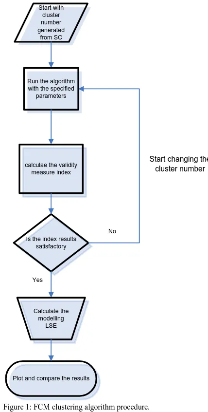
Several parameters must be specified in order to carry FCM algorithm; the number of clusters c, the fuzziness exponent m, the termination tolerance ε, and the norm -inducing matrix A. Finally, the fuzzy partition matrix U must be initialized. The number of clusters c is the most important parameter. When clustering real data without any priori information about the structures in the data, one usually has to make assumptions about the number of underlying clusters. The chosen clustering algorithm then searches for c clusters, regardless of whether they are really present in the data or not. The validity measure approach and iterative merging or insertion of clusters approach are the main approaches used to determine the appropriate number of clusters in data. Figure 1 shows the steps of carrying FCM algorithm.
Start with cluster number generated
from SC
calculae the validity measure index
Is the index results satisfactory Run the algorithm with the specified
parameters
Start changing the cluster number
Plot and compare the results
Figure 1: FCM clustering algorithm procedure.
2.2.Subtractive clustering algorithm:
below a threshold. Although this method is simple and effective, the computation grows exponentially with the dimension of the problem because the mountain function has to be evaluated at each grid point.
Chiu [8] proposed an extension of Yager and Filev’s mountain method, called subtractive clustering.
This method solves the computational problem associated with mountain method. It uses data points as the candidates for cluster centers, instead of grid points as in mountain clustering. The computation for this technique is now proportional to the problem size instead of the problem dimension. The problem with this method is that sometimes the actual cluster centres are not necessarily located at one of the data points. However, this method provides a good approximation, especially with the reduced computation that this method offers. It also eliminates the need to specify a grid resolution, in which tradeoffs between accuracy and computational complexity must be considered. The subtractive clustering method also extends the mountain method’s criterion for accepting and rejecting cluster centres.
The parameters of the subtractive clustering are χi is
the normalized data vector of both input and output
dimensions defined as:
}
total number of data vectors, ra ishyper sphere cluster
radius in data space, rb is the hyper sphere penalty radius
in data space, Pi is the potential value of data vector i, η is
the squash factor =
b a
r
r
,ε
is the accept ratio, andε
isthe reject ratio. The subtractive clustering method works as follows. Consider a collection of n data points
{
x1,x2,x3,...,xn}
in an M dimensional space. Without loss of generality, the data points are assumed to have been normalized in each dimension so that they are bounded by a unit hypercube. Each data point is considered as a potential cluster center. The potential of data point xi isdefined as:
Where, the symbol || . || denotes the Euclidean distance, and ra is a positive constant. Thus, the measure
of the potential for a data point is a function of its distances to all other data points. A data point with many neighboring data points will have a high potential value. The constant ra is effectively the radius defining a
neighborhood; data points outside this radius have little influence on the potential. After the potential of every data point has been computed, we select the data point with the highest potential as the first cluster center. Let x*1 be the
location of the first cluster center and P1* be its potential
value. We then revise the potential of each data point xi by
the formula:
where rb is a positive constant. Thus, we subtract an
amount of potential from each data point as a function of its distance from the first cluster center. The data points
near the first cluster center will have greatly reduced potential, and therefore will unlikely be selected as the next cluster center. The constant rb is effectively the radius
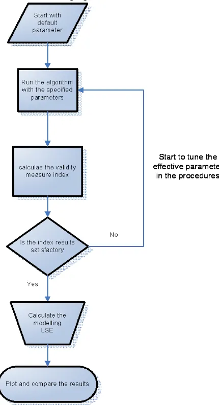
defining the neighborhood which will have measurable reductions in potential. When the potential of all data points has been revised, we select the data point with the highest remaining potential as the second cluster center. This process continues until a sufficient number of clusters are obtained. In addition to these criterions for ending the clustering process are criteria for accepting and rejecting cluster centers that help avoid marginal cluster centers. Figure 2 demonstrates the procedure followed in determining the best clustering results output from the subtractive clustering algorithm.
Figure 2: Subtractive clustering algorithm procedure.
3.Validity Measurement
correctly. When this is not the case, misclassifications appear, and the clusters are not likely to be well separated and compact. Hence, most cluster validity measures are designed to quantify the separation and the compactness of the clusters. However, as Bezdek [6] pointed out that the concept of cluster validity is open to interpretation and can be formulated in different ways. Consequently, many validity measures have been introduced in the literature, Bezdek [6], Dave’s [9], Gath and Geva [10], Pal and Bezdek [11].
3.1.Bezdek index :
Bezdek [6] proposed an index that is sum of the internal products for all the member ship values assigned to each point inside the U output matrix. Its value is between [1/c, 1] and the higher the value the more accurate the clustering results is. The index was defined as:
∑∑
= =In general, an optimal cluster number c* that produces the best clustering performance for the data is found by solving:
3.2.Dave’s Validity Index:
The Dave’s validity index presented in [9] has been successfully used by many researchers. It has an excellent sense to hidden structures inside the data set. Dave’s [9]’s defined the validity measure as:
)
This is a modified version of validity measure VPC
proposed by Bezdek [6]. Dave’s index usually ranges between 0 and 1. The higher the value of the index is, the better the results are. The study by Wang et al [12] reported that VMPC has successfully discovered the optimal
number of clusters in most of the testing benchmarks.
3.3.Xie and Beni Index:
Xie and Beni validity index [13] is defined as:
2
This index has been found to perform well in practice. It can be interpreted as the ratio of the total within-group variance and the separation of the cluster centres. The optimal c* that produces the best clustering performance for the data is found by solving
) , , ( min2≤c≤n−1χ ZUV
4.Results and Discussion
The Fuzzy C-mean algorithm and Subtractive clustering algorithm are implemented to find the number & the position of clusters for a set of highly non-linear data. The clustering results obtained are tested using validity measurement indices that measure the overall goodness of the clustering results. The best clustering results obtained are used to build input/output fuzzy models. These fuzzy models are used to model the original data entered to the algorithm. The results obtained from the subtractive clustering algorithm are used directly to build the system model, whereas the FCM output entered to a Sugeno-type training routine. The obtained least square modeling error results are compared against similar recent researches in this field. When possibility allowed, the same functions and settings have been used for each case.
This section starts with presenting some simple example to illustrate the behavior of the algorithms studied in this paper. Next two highly nonlinear functions are modeled using both algorithms. Finally experimental data are modeled.
4.1.Illustrative cases:
In order to clarify the basic behavior of the two clustering algorithms; three cases are discussed:
4.1.1.Sine wave data modeling
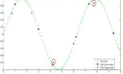
Figure 3 compares between FCM and Subtractive clustering in modeling sine wave data. For this data, Subtractive clustering outperforms the FCM as the eventual goal of the problem is to create a model for the input system. The FCM prototypes are likely to be in the middle area especially in the rounded area as in the peak and the bottom of the sinusoidal wave. This is because the FCM would always estimate the cluster center over a circular data area. When remodeling these prototypes to obtain the original system model, the prototypes generated by the FCM will be shifted outward. As a result, the entire model will be shifted away from the original model. The FCM resulting cluster centers are highlighted by a circle. We can see that subtractive clustering was successful in defining the cluster center because the subtractive clustering assumes one of the original data points to act as the prototype of the cluster center. The resulting subtractive clustering centers are pointed by black box.
4.1.2.Scattered data clustering
The behavior of the two algorithms is tested against scattered discontinuous data. The subtractive still deploy the same criteria to find out the cluster center from the system available points. Thus, it might end to choose relatively isolated points as a cluster center. Figure 4 compares between the two algorithms with scattered data. The suspected points for Subtractive algorithms are circled. However, the FCM still deploy the weighted center. It can reach more reasonable and logical distribution over the data. The performance of the FCM is more reliable for this case.
Figure 4: Scattered points clustering FCM versus Subtractive.
4.1.3.Well separated clusters
In this section, comparison between the two algorithms for clustering well separated clusters is presented. A sample data set provided by Mathwork [50] that contains 600 points distributed in three well defined clusters, are clustered using FCM and Subtractive algorithms. The effect of the number of clusters parameter in the FCM performance is investigated. Also the effect of radii parameters in the Subtractive algorithm is studied. Dave’s, Bezdek and Xi-Beni validity indices variations with number of clusters are calculated and listed.
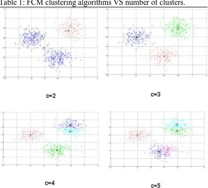
Table 1 lists the results by using FCM with varying number of clusters. It can be easily seen from table 1 that there are three well-defined clusters.
Table 1: FCM clustering algorithms VS number of clusters.
Table 2 list of Dave’s validity index VMPC and Bezdek
indexVPC as a function of number of clusters assigned for
FCM clustering. The parameters like fuzziness m=2, number of iteration =100, and minimum amount of improvement 1*10-5 are used. It can be seen from table 2 that the optimal value for the validity indices obtained when the number of chosen clusters is three, which reflects the natural grouping of the structure inside this data sample.
Table 2: Dave’s validity index VMPC and Bezdek index VPC versus number of clusters c.
Number of clusters c 2 3 4 5
VMPC 0.5029 0.7496 0.6437 0.5656
VPC 0.7514 0.8331 0.7328 0.6500
As discussed earlier, Subtractive algorithm has many parameters to tune. In this study, only the effect of radii parameter has been investigated. Since this parameter has the highest effect in changing the resulting clusters number. Table 3 lists the results by using Subtractive algorithm with varying the radii.
Table 3: Subtractive clustering algorithms Vs radii.
Dave’s validity and Bezdek indices are computed for several values of radii parameter for subtractive clustering. Parameters such as squash factor = 1.25, accept ratio = 0.5 and reject ratio = 0.15 are used. Table 4 lists the radii parameter with the generated number of clusters versus Dave’s validity index VMPC and Bezdek index VPC. It is
apparent from the validity measures that the optimal clustering results are obtained with 3 clusters which generated from using radii = 0.3 units. Even though the radii=0.6 and radii =0.3 generates three clusters, the VMPC
for radii =0.3 is better than that associated with 0.6. Similar behavior is observed for Bezdek validity index.
Table 4: Dave’s validity index VMPC and Bezdek index VPC versus
radii for Subtractive algorithm.
Radii 0.7 0.6 0.3 0.25
Number of clusters c 2 3 3 5
VMPC 0.5071 0.6515 0.7478 0.5715
VPC 0.7536 0.7677 0.8318 0.6572
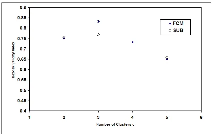
Figure 5: Bezdek validity index Vs number of clusters c for FCM and Sub Algorithms.
Figure 6: Dave’s validity index Vs number of clusters c for FCM and Sub Algorithms.
Figure 7 shows Xi-Beni validity indices variations with number of clusters c for FCM and Subtractive algorithms. Same parameters mentioned previously are used. Although for Subtractive algorithm the same number of cluster are generated for the radii 0.6 and 0.3, the validity measure goes to its optimal value for radii= 0.3.
Figure 7: Xi-Beni validity indices variations with number of clusters c for FCM and Subtractive algorithms.
4.2.Non-linear system modeling:
In this section, several examples are presented in deploying the clustering algorithms to obtain an accurate model of highly nonlinear functions. The models are generated from the two clustering methods. For subtractive clustering the radii parameters are tuned. This automatically generates the number of clusters. The number of clusters is input to the FCM algorithm as starting point only. The generated models is trained using hybrid learning algorithm to identify the membership function parameters of single-output, (Sugeno type fuzzy inference systems FIS). A combination of least- squares and back propagation gradient descent methods are used
for training FIS membership function parameters to model the given model. The training routine is used as a tool to shape out the resulting model and to optimize the rule.
The results obtained from using FCM and Subtractive clustering for example 1 are compared against two recent studied conducted by Alta et al. [3] and Moaqt [4]. Alta et al.[3] used GA to optimize the clustering parameters. Moaqt [4] used 2 nd orders Sugeno consequent system to optimize the resulting model from subtractive clustering algorithm.
Example 1: Modeling the nonlinear function
x
x
y
=
sin
Figure 8 shows a plot of the nonlinear function
x x
sin over two cycles and the optimal resulting generated
model from Subtractive and FCM clustering. Generated models are obtained by using100 clusters for FCM and 0.01 is set for radii parameter for Subtractive algorithm. It can be seen from Figure 8 that both algorithms accurately model the original functions. Table 5 lists the validity measures for subtractive algorithm. Changing the Radii parameter has effectively affects the performance of the algorithm. Generally, lowering the radii parameter has increased the performance measures indices, except for the case of 5 clusters. This is because of the nature of the data considered in this example. Table 6 lists validity measures for the FCM model. Similar behavior is observed for FCM method, that is, as the number of clusters increases, the performance improves. The ** superscript indicates that the index values are undefined but it is approaching 1:
1 '
lim =
→nDavesindex c
and
1
lim =
→nXi-Beni index
c
Figure 8: FCM Vs Subtractive for modeling y=sin(x)/x, 100 clusters.
Table 5: Validity measure for subtractive clustering. Radii
value
Generated number of clusters
Dave’s index
Bezdek index
Dispersion index(XB)
1.1 2 0.6737 0.8369 0.0601
0.9 3 0.6684 0.7790 0.1083
0.5 5 0.6463 0.7171 0.1850
0.02 100 0.8662 0.8676 0.1054
-Table 6: Validity measure for FCM clustering.
Number of assigned clusters
Dave’s index
Bezdek index
Dispersion index(XB)
2 0.7021 0.8511 0.0639
3 0.7063 0.8042 0.0571
5 0.6912 0.7530 0.0596
100 0.8570 0.8487 0.0741
126 NA ~ 1** NA ~ 1** NaN~0**
The Modeling errors are measured through LSE. Table 7 summaries the modelling error from each method and those obtained by Moaqt and Ramini. The LSE obtained by FCM followed by FIS training is 4.8286*10
-9
. On the other hand, the same function is modeled using the subtractive clustering algorithm and the outcome error is 2.2694*10-25. The default parameters with very minimal changes to the radii are used for the subtractive clustering algorithm. The above example was solved by Alata et al. [3] and the best value through deploying Genetic algorithm optimization for both the subtractive parameter and for the FCM fuzzifier is 1.28*10-10. The same problem was solved by H. Moaqt [4]. Moaqt [4] used subtractive clustering to define the basic model and then a 2nd order ANFIS to optimize the rule. The obtained modeling error is 11.3486*10-5.
Table 7: Modeling results for Subtractive Vs FCM.
Example 2: Single-input single-output function
Another nonlinear function
3
sin
x
x
y
=
is modeled byusing subtractive and FCM clustering. Figure 9 shows the original function and output models generated from FCM and Subtractive clustering using 126 clusters. Table 8 lists validity indices (Dave’s index, Bezdek index, and Dispersion index) versus radii parameter for subtractive clustering. Based on the validity measure, table 8 shows that using radii parameter equals to 1.1 that generates two clusters is better than that associated with using 3, 5, or 60 clusters. Optimal representation is obtained when setting radii parameter equals to 0.01 (generated 126 clusters).
Figure 9: Single input function models, FCM Vs Subtractive, 126 clusters.
Table 8: Validity measure Vs cluster parameter for subtractive clustering.
Radii
parameter
Generated
number of
clusters
Dave’s
index
Bezdek
index
Dispersion
index(XB)
1.1 2 0.8436 0.9218 0.0231
0.9 3 0.7100 0.8067 1.1157
0.4 5 0.7010 0.7608 0.6105
0.05 60 0.7266 0.7311 1.1509
0.01 126 1 1 2.1658*10
The same function is modeled using FCM clustering. Table 9 lists the validity measures (Dave’s, Bezdek and Dispersion index) versus number of clusters. Similar behavior to Subtractive clustering is observed when using FCM, such that optimal values associated with using 126 clusters. Table 10 lists the resulting modeling error for both algorithms.
Table 9: Validity measure Vs cluster parameter for FCM clustering.
Number of assigned clusters
Dave’s index
Bezdek
index Dispersion index(XB)
2 0.8503 0.9251 0.0258
3 0.8363 0.8908 0.0300
5 0.7883 0.8307 0.0513
60 0.7555 0.7416 2.7595
110 0.9389 0.9271 0.1953
126 Na~1 Na~1 Na~0
Table 10: Modeling results for subtractive Vs FCM.
Used Algorithm
Number of generated clusters
Output LSE error With training
Output LSE error Without training
FCM 110(user
input) 5.6119*10
-5 2.82*10+5
Subtractive 110 ---- 1.4155*10
-25
4.3.Modeling experimental data:
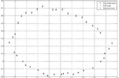
A set of data that represent a real system with an elliptic shaped model obtained from real data experiments [14] is modeled. Figure 10 shows the real data points and the generated models obtained from FCM and subtractive clustering using 38 clusters.
Table 11 summaries the validity measure variations with radii parameter for subtractive clustering. For this set of data, optimal value of validity measure obtained when radii parameter is 0.02. Generally, the smaller the radii parameter is the better the modeling results are. From the table 11, the model generated by using radii =1.1 that generated 2 clusters performed better than that obtained from using three clusters. The reason behind this is that the data is distributed into two semi-spheres (one cluster for each semi-sphere). However, further decrease in the value of Radii improves the resulting model.
Table 11: Validity measure Vs cluster parameter for subtractive clustering.
Radii parameter
Generated number of clusters
Dave’s index
Bezdek
index Dispersion index(XB)
1.1 2 0.5725 0.7862 0.1059
0.9 3 0.5602 0.7068 0.1295
0.5 6 0.6229 0.6858 0.0806
0.05 39 0.9898 0.9895 0.0077
0.02 40 1 1 4.9851*10-25
Table 12 summaries the validity measure variation with the number of clusters using FCM algorithm. Similar behavior to the subtractive clustering is observed.
Table 12: Validity measure Vs cluster parameter for FCM clustering.
Number of assigned clusters
Dave’s index
Bezdek
index Dispersion index(XB)
2 0.5165 0.7582 0.1715
3 0.5486 0.6991 0.1151
20 0.7264 0.7287 0.0895
30 0.8431 0.8395 0.1017
39 0.9920 0.9813 0.0791
40 Na~1 Na~1 Na~0
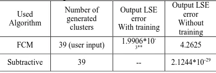
Table 13 compares the LSE error with and without training between FCM and subtractive clustering. It can be seen that FCM algorithm without training routine does not model the data. However, using FCM with training algorithm yields acceptable results. On the other hand, the LSE error resulted from using subtractive algorithm is on the order of 10-29. Double superscript * indicates that the value listed here is an average of 20 different runs.
Table 13: Modeling results for subtractive Vs FCM.
Used Algorithm
Number of generated clusters
Output LSE error With training
Output LSE error Without training
FCM 39 (user input) 1.9906*10
-3** 4.2625
Subtractive 39 -- 2.1244*10-29
5.Conclusion
In this work a comparison study has been performed between FCM clustering algorithm and subtractive clustering algorithm according to their capabilities to model a set of non-linear systems and experimental data. A concise literature review is provided. The basic parameters that control each algorithm are presented as well. The clustering results from each algorithm are assessed using Dave’s, Bezdek, and Xi-Beni validity measurement indices.
For the majority of the system discussed earlier; increasing the number of generated cluster yields an improvement in the validity index value. The optimal modelling results are obtained when the validity indices are on their optimal values. Also, the models generated from subtractive clustering usually are more accurate than those generated using FCM algorithm. A training algorithm is needed to accurately generate models using FCM. However, subtractive clustering does not need training algorithm. FCM has inconsistence problem such that, different running of the FCM yield different results as the algorithm will choose an arbitrary υ matrix each time. On the other hand, subtractive algorithm produce consist results.
The best modelling results obtained for example 1 when setting the cluster number equals to 100 for the FCM and the radii to 0.01. Using these parameter values yields an optimal validity results. The LSE was 4.8286*10-9 for the FCM and 2.2694*10-25 using the subtractive clustering.
For the data in example 2 optimal modelling obtained when using 126 clusters for the FCM and 0.01 radii input for the Subtractive. The LSE are 5.6119*10-5 and 7.0789 *10-21 for the FCM and subtractive respectively. As for the
data in example 3 going to 110 clusters for the FCM and 0.03 radii yields the best clustering results that is, 5.6119*10-5 for the FCM and 1.4155*10-25 for the subtractive clustering. As for experimental data which for an elliptic shape, optimal models obtained when using 39 clusters for FCM. For subtractive clustering, optimal values obtained by setting radii=0.02. The LSE is 1.9906*10-3 and 2.4399*10-28 for the FCM and subtractive respectively.
References
[1] R.O. Duda, P.E. Hart, D.G. Stork, Pattern Classification, 2nd edition, John Wiley, New York; 2001.
[2] Hussein Al-Wedyan, Control of whirling vibrations in BTA deep hole boring process using fuzzy logic modeling and active suppression technique, 2004.
[3] M. Alata, M. Molhim, A. Ramini, “Optimizing of fuzzy C-means clustering algorithm using GA”. Proceeding of world academy of science, Engineering and technology, Vol. 29, 2008, 1307-6884.
[4] H. Moaqt, “Adaptive neuro-fuzzy inference system with second order Sugeno consequent”. Jordan University of science and technology, Master Theses, 2006.
[5] J. C. Dunn, “A fuzzy relative of the Isodata process and its use in detecting compact well-separated clusters”. J. Cybern, 1973, 32-57.
[6] J. C. Bezdek, “Pattern Recognition with Fuzzy Objective Function”. New York, Plenum Press, NewYork, 1981.
[7] R. Yager, D. Filev, “Generation of Fuzzy Rules by Mountain Clustering”. Journal of Intelligent & Fuzzy Systems, Vol. 2(3), 1994, 209-219.
[8] S.L. Chiu, “Fuzzy model identification based on cluster estimation”. J. Intell. Fuzzy Systems, Vol. 2, 1994, 267-278. [9] R.N. Dave, “Validating fuzzy partition obtained through
c-shells clustering”. Pattern Recognition Lett., Vol. 17, 1996, 613–623.
[10] Gath, A. Geva, “Unsupervised optimal fuzzy clustering”. IEEE Transactions on Pattern Analysis and, Machine Intelligence, Vol. 7, 1989, 773–781.
[11] N.R. Pal, and J.C. Bezdek, “On cluster validity for the fuzzy C-means model”. IEEE Trans. on Fuzzy Systems, Vol. 3, 1995, 370–379.
[12] W. Wang, Y. Zhang, “On fuzzy cluster validity indices”. Fuzzy Sets and Systems, Vol. 158, 2007, 2095-2117. [13] Xie X., G. Beni, “Validity measure for fuzzy clustering”.