PAPER
Improving delivery routes using combined heuristic and optimization in a
consumer goods distribution company
To cite this article: E Wibisono et al 2017 IOP Conf. Ser.: Mater. Sci. Eng. 273 012022
View the article online for updates and enhancements.
Improving delivery routes using combined heuristic and
optimization in a consumer goods distribution company
E Wibisono, A Santoso and M A Sunaryo
Department of Industrial Engineering, University of Surabaya, Raya Kalirungkut, Surabaya 60293, Indonesia
E-mail: [email protected]
Abstract. XYZ is a distributor of various consumer goods products. The company plans its delivery routes daily and in order to obtain route construction in a short amount of time, it simplifies the process by assigning drivers based on geographic regions. This approach results in inefficient use of vehicles leading to imbalance workloads. In this paper, we propose a combined method involving heuristic and optimization to obtain better solutions in acceptable computation time. The heuristic is based on a time-oriented, nearest neighbor (TONN) to form clusters if the number of locations is higher than a certain value. The optimization part uses a mathematical modeling formulation based on vehicle routing problem that considers heterogeneous vehicles, time windows, and fixed costs (HVRPTWF) and is used to solve
routing problem in clusters. A case study using data from one month of the company’s
operations is analyzed, and data from one day of operations are detailed in this paper. The analysis shows that the proposed method results in 24% cost savings on that month, but it can be as high as 54% in a day.
Keywords: nearest-neighbor heuristic; vehicle routing problem; heterogeneous vehicles; time windows; consumer goods distributor.
1. Introduction
Logistics operations are oriented toward the fulfillment of customer needs from the point of origin to the point of consumption. One mode of operation in this field is the vehicle routing problem (VRP) that has received considerable attention from academics and practitioners, mainly due to its relevant applications that are often encountered in real world. Being a popular routing model in logistics studies, a number of variants have been developed, tested, and applied. These variants follow the characteristics of the problem being studied, e.g. VRP with time windows (VRPTW) [1], VRP with pickups and deliveries [2], or more specific variants such as VRPTW with evolutionary algorithm [3], VRP with split deliveries [4], or VRP with multiple objectives [5]. More recent VRP studies include, e.g. VRPTW with probabilistic travel times [6], green VRP [7], or VRP in maritime logistics [8].
2
allows more in-depth study of the problem on hand, it deviates from reality in industrial applications. In contrast to the number of general VRP articles cited in [9], only 22 articles related to HVRP were published between 1984 and 2007 [11]. In this particular area where analytical approach is hardly efficient, metaheuristics spur as sensible substitute in dealing with complex VRP problems. A few successful examples worth mentioning are record-to-record [12], scatter search [13], genetic algorithm [14], variable neighborhood search [11], multi-start adaptive memory programming [15], iterated local search [16], and tabu search [17].
This paper demonstrates the application of HVRP in a consumer-goods distribution company operating in Surabaya, Indonesia. Being a large city, there are hundreds of wholesalers and retailers in Surabaya served by the company. The complexity of the problem arises both from the number of customers and the heterogeneity of vehicles (in terms of capacity and fixed cost) that the company uses. Time windows are also demanded by the customers. Thus, the model is called HVRP with time windows and fixed costs (HVRPTWF). Routing of distribution is planned on a daily basis therefore computation time has a higher priority than optimality of the solution. To address the problem complexity, an approach integrating the classical time-oriented, nearest neighbor (TONN) heuristic [18] and optimization via mathematical programming is proposed. This integration is a necessity since mathematical programming alone will clearly be impractical as it will suffer from long computation time on complex problems. The proposed model will be compared to the method that the company applies in its daily operations.
Given the above background, the objectives of this paper are twofold:
To develop an integrated model combining heuristic and optimization in solving routing problem that considers heterogeneous vehicles and time windows.
To compare the solution from the proposed model with the actual routing obtained from the
company’s operations.
2. Methodology
We first described in this section the background of the company in our case study. The company XYZ was founded in 1995 as a distributor of consumer goods products serving mainly the Eastern part of Indonesia. The products varied from toiletries (shampoo etc.) to foods (snacks etc.) and the customers also varied from small retailers to giant hypermarkets. XYZ’s fleet of vehicles comprised more than 300 trucks/vans and 100 motorcycles, operating from 85 branch offices and 25 warehouses in Indonesia. Orders were received daily from sales force then processed by the planning department
to produce delivery plan for the next day. In our study, we focused on Surabaya office (the company’s
headquarters) and the foods division.
XYZ’s customers were classified in three groups: small, large, and super stores. The small stores were served between 8.00 and 13.00, and in Surabaya they were clustered into six areas where each was visited weekly on different days. The large stores were served between 9.00 and 14.00 and clustered into three areas that could be visited every day based on the orders placed. The super stores, given their large demand, had no regular service hours and clusters, and could be served any time
within XYZ’s working hours. This clustering was the basis of XYZ in making its daily distribution plan. Since drivers were already assigned areas of operations, it was possible that two vehicles depart to two different stores, adjacent on the map but on different distribution areas, without maximizing the vehicle capacity (not fully loaded). Often it was possible for these stores to actually be served by the same vehicle, but the drivers who were used to work in specific areas found it uncomfortable to go to different ones. In addition, the planning department only provided the list of stores to be visited
without route and rely on the drivers’ experience to plan their own routes every day. All this led to inefficiency in the operations which was visible from the uneven workload of vehicles where some returned after 12 hours but some did after 18 hours.
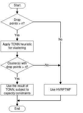
drop points if they exceeded a certain number that prevented the mathematical model HVRPTWF to be run in an acceptable time. Figure 1 shows the path of solution in the methodology.
Start
Drop points > n?
Yes
Apply TONN heuristic for clustering
Cluster(s) with drop points > n?
Yes
Use the result of TONN, subject to capacity constraints
Use HVRPTWF
End
No
No
Figure 1. Solution path in proposed methodology.
Figure 1 is explained as follows. First, customers are grouped into drop points because the number of drop points is what affects the routing instead of the number of customers. If there are less than n
drop points to be served on a particular day, HVRPTWF is applied. If there are more, TONN heuristic is executed to form the clusters and sequence of visit in each cluster. If, after the heuristic, there are still clusters with more than n drop points, the sequence produced by TONN will be used as the route for vehicles serving that route, subject to capacity constraints. It is possible at this stage to divide a TONN cluster into smaller sub-clusters if vehicle capacity is not sufficient to serve all drop points in that cluster. If the heuristic produces clusters with less than n drop points, HVRPTWF is applied in each of such clusters.
The TONN heuristic is explained with the following example. Suppose �is the set of all nodes (locations) including node 0 as depot and� is the set of drop points or � ∖ { }. Given visited exactly prior to , and are the arrival times at nodes and , respectively, � is the service time at node , and , is the travel time from to , then the relationship between and is formulated as
+ � + , , ∀ , ∈ �. The lower and upper time windows at node , and �, respectively,
4
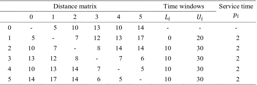
Table 1. Data for Time-Oriented, Nearest-Neighbor heuristic example.
Distance matrix Time windows Service time
�
Given the data in Table 1, the first cluster resulting from the heuristic and its sequence from depot is 0→1→2→3→0 and the second cluster and its sequence is 0→4→5→0. The heuristic only solves
the clustering problem with respect to time windows and leaves the capacity allocation to the second part in methodology, i.e. mathematical programming with HVRPTWF. In Figure 1, the value of n will be determined after few trial runs of HVRPTWF to see at how many nodes the model becomes impractical with regard to computation time. In the above example, suppose it is found that n = 2 (this low figure is only for the sake of this example), then the first cluster will not be optimized with HVRPTWF and the heuristic result will be used with arbitrary vehicle assignment.
For HVRPTWF, the mathematical model follows [19] with more specific elaboration on the lower time window (in [19] the model is applied on maritime logistics case and only the upper time window which reflects due date is used). The sets and equations are explained in the following.
∑��, fixed costs of using vehicles. Demand fulfillment is warranted by constraints (2) and vehicle capacity is observed by constraints (3). Constraints (4) balance the incoming and outgoing flows. Constraints (5) are loop prevention and constraints (6) regulate so that a vehicle can take only one trip. Constraints (7) set the lower and upper time windows for a vehicle at a node, while constraints (8) manage the arrival times similar to the explanation in the heuristic section. Sub-tour breaking constraints are not required due to constraints (8). Lastly, constraints (9)–(11) state the nature of decision variables involved:��, are binary and � are continuous, thus the model falls in the category MILP problem.
3. Case study analysis
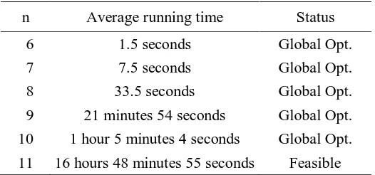
Our first step in analysis was determining the threshold n to limit the number of drop points that HVRPTWF could still solve efficiently. Using a commercial solver and Intel Core i5 processor running at 2.2 GHz with 4GB RAM on Windows 10, we arrived at the results in Table 2. From this table it can be inferred that n should be set equal to 10. With more than 10 locations, the solver was still unable to find an optimal solution after more than 16 hours.
Table 2. Computation time of HVRPTWF.
11 16 hours 48 minutes 55 seconds Feasible
Next, a sample of one-month company’s operation in the foods division was studied. In this section, we provided an example of one-day distribution and compared the results between the
company’s method and our proposed methodology combining TONN heuristic and HVRPTWF
6
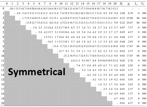
Table 3. Distance matrix (km), demands (m3), service time and time windows (mins) of locations.
0 1 2 3 4 5 6 7 8 9 10 11 12 13 14 15 16 17 18 19 20 Di pi Li Ui
0 - 20.1 13.5 14.7 19.0 20.0 18.4 18.3 18.4 18.5 12.7 24.5 21.4 18.7 17.5 19.8 18.8 18.7 16.7 18.3 13.3 - - - - 1 - 6.6 5.4 11.9 11.5 11.4 11.2 4.5 11.4 7.4 19.5 15.2 10.2 10.3 10.3 11.7 11.6 9.5 9.9 9.4 2.08 8.70 0 300 2 - 1.7 15.5 14.0 15.1 14.9 5.2 15.1 4.2 22.0 17.6 12.7 14.0 12.7 15.4 15.3 13.2 12.4 10.5 0.23 25.00 60 360
3 - 13.8 12.7 13.4 13.2 4.6 13.4 2.5 21.0 16.7 11.3 12.3 11.5 13.7 13.6 11.5 11.1 9.8 0.22 25.67 60 360 4 - 3.4 2.5 2.3 14.4 2.5 13.7 10.5 6.5 3.7 1.6 3.1 2.8 2.7 2.4 3.3 5.7 0.07 7.37 0 300 5 - 3.8 4.2 13.7 3.1 13.0 10.6 6.6 3.0 3.8 2.4 4.2 2.9 3.3 2.7 2.7 0.05 4.37 0 300 6 - 1.5 15.1 1.7 14.4 8.6 4.6 4.4 2.4 3.8 0.4 1.8 2.1 4.1 6.0 0.04 2.37 0 300
7 - 14.5 1.1 13.3 10.1 5.7 4.8 1.6 4.2 1.3 1.3 2.5 4.5 4.0 0.04 2.03 0 300 8 - 13.4 5.7 21.3 16.9 12.0 12.9 12.0 14.7 13.3 13.0 11.6 10.8 0.03 17.67 60 360 9 - 13.7 9.1 5.1 3.9 1.1 3.3 1.3 0.2 2.3 3.5 5.2 0.03 2.37 0 300 10 - 21.2 16.9 11.7 12.6 11.7 14.0 13.6 12.3 11.4 8.8 0.02 17.67 60 360
11 - 4.4 11.3 9.2 10.7 8.8 8.9 10.0 10.9 12.4 0.02 2.70 0 300 12 - 7.4 5.7 6.9 4.9 4.9 6.7 7.1 8.2 0.02 2.03 0 300 13 - 3.2 1.6 4.3 3.8 4.1 1.9 7.0 0.01 3.37 0 300
14 - 4.2 2.0 1.3 2.9 4.5 4.8 0.01 2.03 0 300
15 - 4.2 3.4 5.3 1.9 8.2 0.01 3.03 0 300
16 - 1.4 2.5 3.7 5.6 0.01 2.03 0 300
17 - 2.5 3.4 5.4 0.01 2.37 0 300
18 - 3.4 4.9 0.01 3.37 0 300
19 - 6.7 0.01 2.37 0 300
20 - 0.01 4.37 0 300
Table 4. Data of vehicles.
Type Units Capacity (m3) Cost/day (IDR) Cost/km (IDR)
A 2 2.4 544,687 812.50
B 1 5.6 502,526 812.50
C 1 9.6 603,725 812.50
Using the company’s method, three vehicles were used with the following routings: Vehicle A1: 0→2→3→8→10→0
Vehicle A2: 0→20→6→7→9→16→4→14→17→5→13→15→18→19→12→11→0
Vehicle C: 0→1→0
The above routing demonstrated inefficient use of vehicle C since, despite its large capacity; it was used to serve one particular store simply because that customer had regularly been served by vehicle C and its driver. This one-on-one relationship between customer and driver familiarized the driver with his region of operations. The driver’s knowledge on his region helped on some days and was justified when demand size matched vehicle capacity, but more often led to inefficiency as shown above. The routes constructed by the drivers also relied on their judgment and experience, but was proven
suboptimal compared to the output of heuristic and mathematical programming as outlined in the next section.
4. Results and discussion
Applying the algorithm in Figure 1 yielded the following results. First, two clusters (instead of three) were formed. The first cluster consisted of 15 locations and the second cluster consisted of 5 locations. For the first cluster, total demand was 0.34 m3 so it could be served by vehicle A (time windows had already been taken care of by the heuristic). For the second cluster, HVRPTWF was applied, and it produced a different routing from the actual one by the driver. The routings in both clusters were given below:
Vehicle A1: 0→20→14→9→17→7→16→6→18→4→15→13→19→5→12→11→0
Vehicle B: 0→2→3→1→8→10→0
It is worth to mention here that since we knew from the data that vehicle A could not be used due to its lower capacity (2.4 m3) than the second cluster’s demand (2.58 m3), and vehicle B’s daily cost
was smaller than vehicle C’s, then vehicle B was a logical choice for serving the second cluster.
Further, since time windows were no longer an issue as a result from the heuristic application, routing problem of the second cluster was actually reduced to a travelling salesman problem (TSP). This advantage, however, was not apparent on other cases in different days, so HVRPTWF formulation was still required. Besides, with less than 6 locations, HVRPTWF required not more than 1.5 seconds to solve.
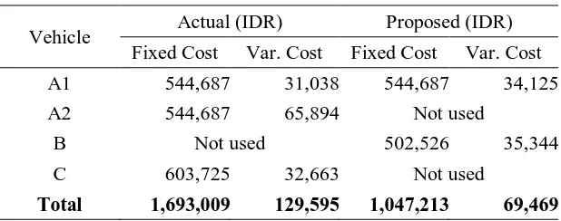
Next, we compared the total cost of actual operations and that of our proposed methodology. As shown in Table 5, the proposed method combining heuristic and mathematical programming was
superior compared to the drivers’ assignment-based method from the company. The proposed method reduced the number of vehicles required that led to cost savings in fixed and variable costs. The cost savings in fixed cost, however, were only on paper since fixed cost was calculated based on
depreciation, drivers’ salaries, etc., i.e. it would be incurred regardless of vehicle utilization. The savings in variable cost, on the other hand, were tangible. For this day only, the savings in variable
cost were 53.60%. For the overall month, the company’s method yields IDR 2,406,548 whereas the
proposed method did IDR 1,849,893 or equivalent to a 23.56% cost reduction.
Table 5. Cost comparison of two methods.
Total 1,693,009 129,595 1,047,213 69,469
5. Conclusions and remarks for future research
In this paper we have demonstrated an application of combined heuristic and optimization to solve practical routing problems in a distribution company. The company planned its delivery routes daily so a methodology that could arrive at good solution in an acceptable time would have a high practical
value. Our proposed approach beat the company’s method that was based on drivers’ regional
8
The comparison in this paper was only made against the actual routings used by the company. It is possible there are still better approaches, be they heuristics or optimization, which should be aimed as future research agenda.
References
[1] El-Sherbeny N A 2010 Vehicle routing with time windows: An overview of exact, heuristic and metaheuristic methods J. King Saud University – Science 22 pp 123–131
[2] Wassan N A and Nagy G 2014 Vehicle routing problems with deliveries and pickups: Modelling issues and meta-heuristics solution approaches Int. J. Transportation 2 pp 95–110 [3] Bräysy O, Dullaert W and Gendreau M 2005 Evolutionary algorithm for the vehicle routing
problem with time windows J. Heuristics 10 pp 587–611
[4] Archetti C and Speranza M G 2012 Vehicle routing problems with split deliveries Int. T. Oper. Res. 19 pp 3–22
[5] Josefowiez N, Semet F and Talbi, E-G 2008 Multi-objective vehicle routing problems Eur. J.
Oper. Res. 189 pp 293–309
[6] Agra A, Christiansen M, Figueiredo R, Hvattum L M, Poss M and Requejo C 2013 The robust vehicle routing problem with time windows Comput. Oper. Res.40 pp 856–866
[7] Lin C, Choy K L, Ho G T S, Chung S H and Lam H Y 2013 Survey of green vehicle routing problem: Past and future trends Expert Syst. Appl. 1 pp 1118–38
[8] Wibisono E and Jittamai P 2015 Collaborative capacity sharing in liner shipping operations Int. J. Logistics Systems and Management 22 pp 520–539
[9] Eksioglu B, Vural A V and Reisman A 2009 The vehicle routing problem: A taxonomic review
Comput. Ind. Eng.57 pp 1472–83
[10] Braekers K, Ramaekers K and Van Nieuwenhuyse I 2016 The vehicle routing problem: State of the art classification and review Comput. Ind. Eng.99 pp 300–313
[11] Imran A, Salhi S and Wassan N A 2009 A variable neighborhood-based heuristic for the heterogeneous fleet vehicle routing problem Eur. J. Oper. Res.197 pp 509–518
[12] Li F, Golden B and Wasil E 2007 A record-to-record travel algorithm for solving the heterogeneous fleet vehicle routing problem Comput. Oper. Res.34 pp 2734–42
[13] Belfiore P and Yoshizaki H T Y 2009 Scatter search for a real-life heterogeneous fleet vehicle routing problem with time windows and split deliveries in Brazil Eur. J. Oper. Res.199 pp 750–758
[14] Prins C 2009 Two memetic algorithms for heterogeneous fleet vehicle routing problems Eng. Appl. Artif. Intel.22 pp 916–928
[15] Li X, Tian P and Aneja Y P 2010 An adaptive memory programming metaheuristic for the heterogeneous fixed fleet vehicle routing problem Transport. Res. E-Log.46 pp 1111–27 [16] Subramanian A, Penna P H V, Uchoa E and Ochi L S 2012 A hybrid algorithm for the
Heterogeneous Fleet Vehicle Routing Problem Eur. J. Oper. Res.221 pp 285–295
[17] Jiang J, Ng K M, Poh K L and Teo K M 2014 Vehicle routing problem with a heterogeneous fleet and time windows Expert Syst. Appl.41 pp 3748–60
[18] Solomon M M 1987 Algorithms for the vehicle routing and scheduling problems with time window constraints Oper. Res. 35 pp 254–265
[19] Wibisono E 2016 Application of genetic algorithm in containerships network design problem