DOI: http://dx.doi.org/10.17509/ijost.v3i1.10799 p- ISSN 2528-1410 e- ISSN 2527-8045
Prediction and Classification of Low Birth Weight Data
Using Machine Learning Techniques
Alfensi Faruk 1*, Endro Setyo Cahyono 1, Ning Eliyati1, Ika Arifieni1
1 Department of Mathematics, Faculty of Mathematics and Natural Science, Sriwijaya University, 30662,
Indralaya, South Sumatra, Indonesia.
*Correspondence: E-mail: [email protected]
A B S T R A C T S A R T I C L E I N F O
Machine learning (ML) is a subject that focuses on the data analysis using various statistical tools and learning processes in order to gain more knowledge from the data. The objective of this research was to apply one of the ML techniques on the low birth weight (LBW) data in Indonesia. This research con-ducts two ML tasks, including prediction and classification. The binary logistic regression model was firstly employed on the train and the test data. Then, the random approach was also applied to the data set. The results showed that the bi-nary logistic regression had a good performance for predic-tion, but it was a poor approach for classification. On the other hand, random forest approach has a very good perfor-mance for both prediction and classification of the LBW data set.
© 2018 Tim Pengembang Jurnal UPI
Article History:
Received 19 November 2017 Revised 03 January 2018 Accepted 01 February 2018 Available online 09 April 2018
____________________
In the last couple of decades, data mining rapidly becomes more popular in many areas such as finance, retail, and social media (Firdaus, et al., 2017). Data mining is an interdisciplinary field, which is affected by other disciplines including statistics, ML, and database management (Riza, et al., 2016). Data mining techniques can be used for various types of data, such as time series data (Last, et al., 2004) and spatial data (Gunawan,
et al., 2016).
Although ML and statistics are two different subjects, there is a continuum between both of them. The statistical test can be used as a validation tool in ML modelling. Furthermore, statistics evaluate the ML algorithms. ML is commonly defined as a subject that focuses on the data-driven and computational techniques to conduct inferences and predictions (Austin, 2002).
Data analysis depends on the type of the data. For instance, the LBW data, which the dependent variable has two values, are
frequently analyzed by using binary logistic regression model. Meanwhile, in machine learning, the traditional binary logistic regression model is modified by including learning process in the analysis. In ML approach, the data were split into two groups, i.e. train data and test data. Some examples of popular ML techniques are support-vector machines, neural nets, and decision tree (Alpaydin, 2010). One of the examples for the use of ML process is in mild dementia data (Chen & Herskovits, 2010)
In this research, the ML techniques based on the ML workflow on the LBW data hat were obtained In particular, the ML techniques are binary logistic regression and random forests. The ML workflow of this research including data exploration, data cleaning, model building, and presenting the results. The computational procedures were conducted by using R-3.3.2 and RStudio version 1.0.136. These softwares are so popular recently because it is a high-quality,
cross-platform, flexible, and open source (Makhabel, 2015).
2. METHODS 2.1. Data
This research used the data set of LBW that were occupied from the result of 2012 Indonesian Demographic and Health Survey (IDHS).
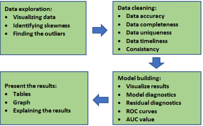
2.2. ML Workflow
The workflow is a series of systematic steps of a particular process. The ML workflow can be in various forms, but it generally consists of four steps, i.e. data exploration, data cleaning, model building, and presenting the results. Every step consists of at least one task. For example, data visualization and finding the outliers are the tasks in data exploration. The determination of the tasks in each ML workflow step depends on the data characteristics and the purposes of the research. The ML workflow of this work is depicted in Figure 1.
DOI: http://dx.doi.org/10.17509/ijost.v3i1.10799 p- ISSN 2528-1410 e- ISSN 2527-8045 2.2. Binary logistic regression.
Binary logistic regression is a type of logistic regression, which has only two categories of outcomes. It is the most simple type of logistic regression. The main goal of binary logistic regression is to find the formula of the relationship between dependent variable Y and predictor X. The form of the binary logistic regression is (Kleinbaum & Klein, 2010):
� � = + exp � + � + ⋯ + �exp � + � + ⋯ + ��
�
where � � is theprobability of the outcome,
� , � , . . . , �� are the unknown parameters, and , , . . . , � are the predictors or independent variables. In ML, binary logistic regression can be used to do prediction and classification.
2.3. Random forests
Random forests are defined as the combination of tree predictors such that each tree depends on the values of a random vector sampled independently and with the same distribution for all trees in the forest (Breiman, 2001). This approach is very common in ML and can also be used for prediction and classification as in binary logistic regression. The steps in the algorithm of the random forests are (Liaw & Wiener,
3. RESULTS AND DISCUSSION 3.1. Description of LBW data
LBW is defined as a birth weight of an in-fant of 2499 g or less. Recently, LBW gets more intentions from many governments over the world because it is one of significant factors that may increase under-five mortality and infant mortality. In this research, the LBW data were obtained from the result of 2012 IDHS. In the beginning, the raw data consists of 45607 women aged 15-49 years as the respondents. After data cleaning process, the amount data reduced to 12055 women aged 15-49 years who give birth from 2007 up to 2012.
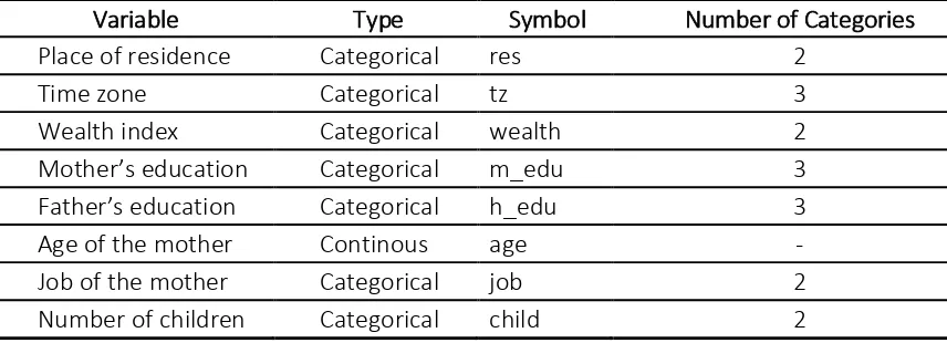
In this work, there are two types of varia-bles, i.e. dependent variable and independent variable. The chosen of the variables based on the other published works (Dahlui et al., 2016; Tampah-Naah et al., 2016). The dependent variable is LBW, which has two categories, i.e. = if a woman gives birth an infant of 2499 g or less otherwise = . Furthermore, the LBW is symbolized as lbw. There are eight independent variables that were chosen and it is summarized in Table 1.
Variable Type Symbol Number of Categories
Place of residence Categorical res 2
Time zone Categorical tz 3
Wealth index Categorical wealth 2
Mother s edu ation Categorical m_edu 3
Father s edu ation Categorical h_edu 3
Age of the mother Continous age -
Job of the mother Categorical job 2
Number of children Categorical child 2
3.2. Data exploration
According to ML workflow in Figure 1, the subsequent phase after getting the data set is to employ exploratory data analysis on the data. The data exploration consists of several common tasks, such as visualizing data distribution, identifying skewness of the data, and finding the outliers. The use of the tasks depends on the data characteristics and the modelling technique. In this research, all the three tasks are committed.
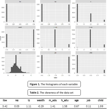
The first step is visualizing the data distributions for all variables. There are two most popular techniques to visualize the data distribution, that is histograms and density plots. Some people prefer using histograms because it provides better information on the exact location of the data. In addition, histograms are also the powerful techniques to detect the outliers. Therefore, this work only employed the histograms as shown in Figure 2.
The histograms in Figure 2 do not indicate that the data for all variables follow the bell-shaped pattern. In other words, the data of each variable are not normally distributed. These results will not affect the model build-ing phase because the binary logistic regres-sion model, which is used in this research, does not assume the normality in the data as in linear regression.
The histograms can also identify the outli-ers in the data set. Therefore, the subsequent step in data exploration is outlier identifica-tion using the histograms. It can be seen from Figure 2 that there are outlier data in several variables including lbw, tz, m_edu, h_edu, and
child. However, because the information from
the outliers is important to achieve the objec-tives of this research, then the outlier data are not removed from the data set.
The last step in data exploration is the skewness identification. The skewness can be defined as a measure of the asymmetry of a data distribution. In this research, the skewness of each variable is calculated by
using ‘ pa kage e1071 and sapply() function.
The result of the calculation can be seen in Table 2.
A skewness that equal to zero indicates a symmetrical distribution of the data. Therefore, a skewness near to zero shows that the data approximate the symmetrical distribution. Moreover, if the absolute value of skewness is more than one, then the skewness of the variable can be categorized as high. According to the skewness values in Table 2, some of the variables have relatively low skewness including res, wealth, age, and job.
3.3. Data cleaning
In data analysis, the objective of data cleaning is commonly used to keep the quality of the data before the data become the inputs in the model building phase. Some aspects of data cleaning that should be considered are the data accuracy, data completeness, data uniqueness (no duplication), data timeliness, and the data consistency (coherent).
Because the data are based on one of the DHS surveys, which are globally used by many researchers and regularly conducted by many governments and USAID for several decades, then the data integrity is highly trustworthy. In this research, the raw data have some missing values and duplicated data. The missing values were already deleted in order to keep the completeness of the data. Meanwhile, the duplicated data were fixed by just using one data for the same recorded data.
DOI: http://dx.doi.org/10.17509/ijost.v3i1.10799 p- ISSN 2528-1410 e- ISSN 2527-8045 that this data set is already timeliness. The
data contain nine variables, that is one dependent variable and eight independent variables. All of these variables are chosen based on the other works and some relevant
references. In other words, the variables have been proved to include in the analysis. This means that the data are already coherent and fit to the research purposes.
lbw res tz wealth m_edu h_edu age job child
3.42 0.03 1.11 -0.29 1.41 1.58 0.67 0.11 1.99
3.3. Data cleaning
Model building is the main process of the ML workflow. In data mining, model building consists of several tasks such as result visualization, model diagnostics, residual diagnostics, ROC curves, etc. In this section, several tasks related to the model building for Indonesian LBW data are discussed, including
result visualization, model and residual diagnostics, multicollinearity checking, misclassification error calculation, plotting the receiver operating characteristic (ROC) curves, and calculation of the area under the curve (AUC).
One of the fundamental differences between traditional statistics and data mining
Figure 1. The histograms of each variable variables
is the using of machine learning. Traditional statistics do not use machine learning in analyzing the data, whereas data mining employs machine learning in addition to some traditional statistical tools and database management.
In the model building phase of ML workflow, the data are firstly split into two groups of data sets, that is training data and test data. It is common that the training data contains about 70-80% of all the data. Meanwhile, about 20-30% of the rest of the data were left as the test data. In this work, the first 80% of the data became the training data and the rest 20% became the test data. After the original data set was split, the binary logistic regression model was fitted to the train data. The estimation procedure for train data was conducted by performing R software
and glm() function.
Before conducting the estimation, the multicollinearity among independent
variables should be checked.
Multicollinearity indicates the excessive correlation among independent variables. One of the problems due to the existence of multicollinearity is the inconsistent results from forward or backward selection of variables.
The variance inflation factors (VIF) is a
simple technique to identify the
multicollinearity among independent variables. The higher the VIF value, the higher the multicollinearity. If the VIF value is more than 4, then it can be said that the VIF value
is high. The pa kage car and vif() function in
R can calculate the VIF value among independent variables. The results of multicollinearity checking and the estimation results for train data are shown in Table 3 and Table 4, respectively.
Table 3 shows that the VIF values for all independent variables are near to one. It means that there is no multicollinearity among independent variables in train data set. Therefore, the analysis can be continued to parameter estimation. The parameter estimation results can be seen in Table 4.
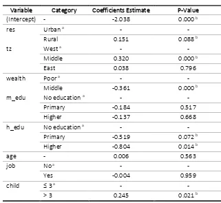
The estimation results in Table 4 show
Variable VIF Value Degree of Freedom (DF)
res 1.201 1
DOI: http://dx.doi.org/10.17509/ijost.v3i1.10799 p- ISSN 2528-1410 e- ISSN 2527-8045
Variable Category Coefficients Estimate P-Value
(Intercept) - -2.038 0.000 b
b. Significant at 10% level
After the estimation results are obtained, the next step in model building is to perform residual diagnostics and model diagnostics. The residual diagnostics consist of several tasks, i.e. deviance analysis and calculation of
r-squared. Meanwhile, model diagnostics can be done by assessing the predictive ability of the model, multicollinearity checking, misclassification error calculation, ROF curve, and AUC.
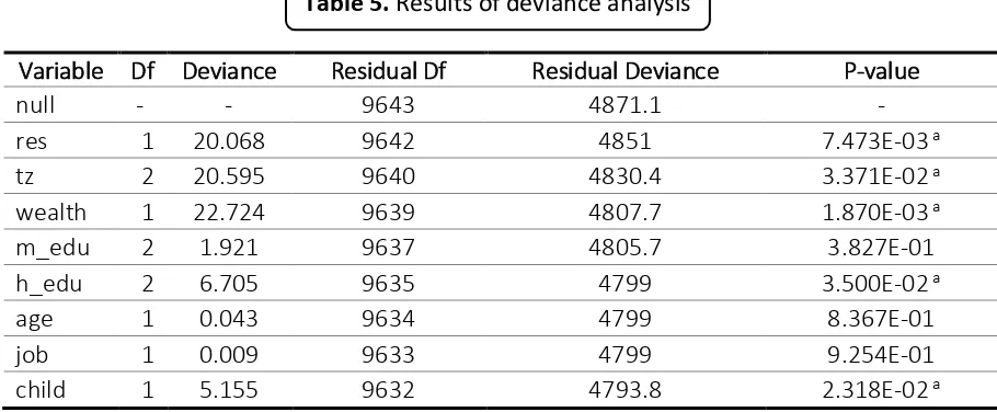
In R, deviance analysis for binary logistic regression can be employed by using anova() function. This analysis performs chi-square statistic to test the significance of the variable in reducing the residual deviance. The deviance analysis for the train data is described in Table 5.
The difference between null deviance value and residual deviance indicates the
performance of the current model against the null model, which only consists of the intercept. The wider gap shows the better model. It can be seen in Table 5 that the residual deviance is decreased along with the adding of independent variables into the model. The widest gap between null model and current model happens when all variables are added into the null model, that is 4871.1-4793.8 = 77.3. In other words, the goodness of fit of the model is increased by adding more independent variables into the null model. From Tabel 5, it can be seen also that there are five variables which significantly reduced the residual deviance at 5% level, i.e.
res, tz, wealth, h_edu, and child.
In the binary logistic regression model, residual diagnostics can be done by calculating the r-squared value. However, R
only calculates the pseudo-r-squared value instead of the exact value of r-squared. In this research, the types of pseudo-r-squared are limited to only three values, i.e. M Fadden s pseudo r-squared (McFadden), maximum likelihood pseudo r-squared (r2ML), Cragg
and Uhler s pseudo-r-squared (r2CU). These
calculate the three pseudo-r-squared for the LBW data set. The calculation with R yields McFadden = 0.016, r2ML = 0.008, and r2CU = 0.02. The model has a good fit to the data if the McFadden value is between the range of 0.2-0.4. Although the McFadden value does not lie in that range, all three pseudo-r -squared values are very close to zero. These small r-squared values indicate that the error of the model is very small. In other words, the model is acceptable as a good fit.
After evaluating the fitting of the model, another task that should be done is to asses the predictive ability of the model. The goal is
to see how the model is doing when predicting Y on the test data. By using R, the output probability has the form Pr = | . In this work, 0.5 is chosen as the threshold. It means that if Pr = | > .5, then = prediction accuracy of the test data is a good result.
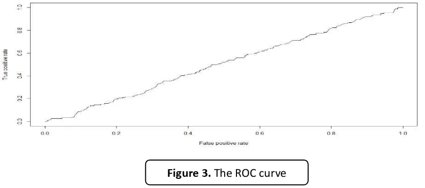
The final tasks for model building in this research are plotting the ROC curve and several threshold values. Meanwhile, the area under the ROC curve is called AUC. If the AUC is closer to 1 than 0.5, the predictive ability of
the is good. By using pa kage R2OC and
some related functions in R, such as predict(),
prediction(), performance(), and plot(), the
ROC curve can be seen in Figure 3.
Variable Df Deviance Residual Df Residual Deviance P-value
null - - 9643 4871.1 -
DOI: http://dx.doi.org/10.17509/ijost.v3i1.10799 p- ISSN 2528-1410 e- ISSN 2527-8045 The ROC curve in Figure 3 shows that the
performance of binary logistic regression model in classification task is very poor or worthless. This result is also supported by the
AUC value = 0.505, which is so close to 0.5 and
indicates the very poor model for classification.
Because the ROC curve and AUC show that the performance of binary logistic regression model in classification task is very poor, then an alternative model is needed to obtain the better result. In this research, random forest approach is chosen as the alternative classification model. In such approach, a large number of decision trees are constructed. Each observation is fed into the decision trees. The most general outcome of all observations is employed as output. The error estimate in the random forest is called out of bag (OOB) which is commonly represented in percentage.
To conduct the random forest, package
“randomForest and pa kage “party should
be installed into R. By choosing 500 as the number of trees, the random forest for the train data shows that the model has only 7% error, which means that the prediction has 93% accuracy. Based on this result, it is very
recommended to use random forest
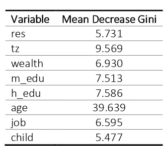
approach instead of binary logistic regression in the classification process. In addition, the random forest also concludes that age of the mother is the most important factors affecting the LBW case. The complete results of the importance of each independent variable are shown in Table 6. In the random forest approach, the higher value of mean decrease gini, the higher the importance of the variable. As shown in Table 6, the mean decrease gini of age has the highest score among the other variables.
Variable Mean Decrease Gini
res 5.731
tz 9.569
wealth 6.930
m_edu 7.513
h_edu 7.586
age 39.639
job 6.595
child 5.477
4. CONCLUSION
In this research, the ML process was applied to the LBW data in Indonesia. The steps including data exploration, data cleaning, model building, and presenting the results. The prediction performance of binary logistic regression model for LBW data was very good. However, the binary logistic regression model failed for LBW data classification. It was indicated by the poor ROC curve and AUC value. On the other hand, the results showed that the random forest approach was highly recommended for both prediction and classification of the LBW data set. Suggestion for further research is to use the other approaches in machine learning, such as conditional tree model and support
vector machines (SVM), in order to find the best approach for classification the LBW data.
5. ACKNOWLEDGEMENTS
This project was sponsored by Sriwijaya University through Penelitian Sains dan Teknologi (SATEKS) 2017. The authors are thankful to United States Agency for International Development (USAID) for con-tributing materials for use in the project.
6. AUTHO‘S NOTE
The authors declare that there is no con-flict of interest regarding the publication of this article. Authors confirmed that the data and the paper are free of plagiarism.
7. REFERENCES
Alpaydin, E. (2010). Introduction to machine learning (2nd ed.). The MIT Press.
Austin, M. P. (2002). Spatial prediction of species distribution: an interface between ecological theory and statistical modelling. Ecological modelling, 157(2-3), 101-118.
Breiman, L. (2001). Random forests. Machine Learning, 45, 5-32.
Chen, R., and Herskovits, E.H. (2010). Machine-learning techniques for building a diagnostic model for very mild dementia. Euroimage, 52(1), 234–244.
Dahlui, M., Azahar, N., Oche, O. C., and Aziz, N. A. (2016). Risk factors for low birth weight in nigeria: evidence from the 2013 Nigeria demographic and health survey. Global Health
Action, 9, 28822.
Firdaus, C., Wahyudin, W., & Nugroho, E. P. (2017). Monitoring System with Two Central Facilities Protocol. Indonesian Journal of Science and Technology, 2(1), 8-25.
DOI: http://dx.doi.org/10.17509/ijost.v3i1.10799 p- ISSN 2528-1410 e- ISSN 2527-8045
Gunawan, A. A. S., Falah, A.N., Faruk, A., Lutero, D.S., Ruchjana, B.N., and Abdullah, A. S. (2016). Spatial data mining for predicting of unobserved zinc pollutant using ordinary point kriging. Proceedings of International Workshop on Big Data and Information Security
(IWBIS), 2016, 83-88.
Kleinbaum, D.G, and Klein, M. (2010) Logistic regresion a self-learning text (3rd ed). Springer.
Last, M., Kandel, A., and Bunke, H. (2004). Data mining in time series databases. World Scientific Publishing Co. Pte. Ltd.
Liaw, A., and Wiener, M. (2002). Classification and regression by random forest. R News, 2(3), 18-22.
Makhabel, B. (2015). Learning data mining with R. Packt Publishing Ltd.
Riza, L. S., Nasrulloh, I. F., Junaeti, E., Zain, R., and Nandiyanto, A. B. D. (2016). gradDescentR: An R package implementing gradient descent and its variants for regression tasks.
Proceedings ofInformation Technology, Information Systems and Electrical Engineering
(ICITISEE), 2016, 125-129.