FORECASTING DAILY AND SESSIONAL RETURNS OF THE
ISE-100 INDEX WITH NEURAL NETWORK MODELS
YAPAY SİNİR AĞLARI MODELLERİ İLE İMKB-100 ENDEKSİNİN GÜNLÜKVE SEANSLIK GETİRİLERİNİN TAHMİN EDİLMESİ
Emin AVCI
Marmara University, Department of Business Administration
ABSTRACT:Especially for the last decade, the neural network models have been
applied to solve financial problems like portfolio construction and stock market forecasting. Among the alternative neural network models, the multilayer perceptron models are expected to be effective and widely applied in financial forecasting. This study examines the forecasting power multilayer perceptron models for daily and sessional returns of ISE-100 index. The findings imply that the multilayer perceptron models presented promising performance in forecasting the ISE-100 index returns. However, further emphasis should be placed on different input variables and model architectures in order to improve the forecasting performances.
Keywords: Artificial neural network models, Stock market forecasting.
ÖZET: Özellikle son on yılda yapay sinir ağları modelleri portföy oluşturma ve hisse senedi piyasası tahminleri gibi finansal problemleri çözmede uygulanmaktadır. Çeşitli yapay sinir ağları modelleri arasında, çok-katmanlı
pörseptron modelleri finansal tahmin çalışmaları için yaygın ve etkili bir şekilde kullanılmaktadır. Bu çalışma, çok-katmanlı pörseptron modellerinin İMKB-100 endeksinin günlük ve seanslık getirilerinin tahmin edilmesindeki etkinliğini incelemektedir. Çalışmanın bulgularından yola çıkılarak, çok-katmanlı pörseptron modellerinin İMKB-100 endeks getirisini tahmin etmede umut vaat eden bir performans gösterdiği sonucuna varılabilir. Fakat, yapay sinir ağları modellerinin tahmin güçleri farklı değişkenler ve farklı model yapıları kullanılarak daha da arttırılabilir.
Anahtar kelimeler: Yapay sinir ağları modelleri, Hisse senedi piyasası tahminleri.
1. Introduction
The elasticity and adaptability advantages of the artificial neural network models have attracted the interest of many researchers from different disciplines including the electrical engineering, robotics and computer engineering, oil and medicine industries. For the last decade, the artificial neural network models have been heavily used in the fields of business, finance and economics for several purposes like time series forecasting and performance measurement.
Among the alternative of artificial neural network models, the multilayer perceptron models with backpropagation algorithm are excepted to be effective and widely applied in financial applications. Among the variety of researchers, Gately (1996) stated that the most commonly used neural network model had been the multilayer perceptron model with backpropagation algorithm. About 85% percent of all applications of neural network models in finance were trained with backpropagation
algorithm. In the same manner, Adya and Collopy (1998) examined the literature for applications of neural network models in business forecasting and prediction during 1988 and 1994. They stated that 88% of the studies used backpropagation as the learning algorithm. In addition, Fadlalla and Lin (2001) examined 40 articles, which were frequently cited in literature on neural networks in finance, published during 1986-1997. They reported that 26 out of 40 were trained by the multilayer perceptron models with backpropagation algorithm, while in 9 of the articles the training methodology was not reported. In related study, Vellido, et al. (1999) investigated the neural network literature in the areas of accounting and finance, management decision-making, marketing and production during the periods 1992-1998. They stated that 74 (out of 93) papers relied on the multilayer perceptron trained by the backpropagation algorithm. Moreover, they pointed out that the backpropagation algorithm became a standard operation for supervised learning in neural network models. And also, Thawornwong and Enke (2003) examined 45 journal articles published from 1996 to 2002 about the neural network applications for financial markets. They also stated that approximately 82% of the studies (37 out of 45) used the backpropagation algorithm.
Relying on the outstanding performance of multilayer perceptron models with backpropagation algorithm in financial applications, this study aimed at investigating the forecast performance of the multi-layer perceptron models on daily and sessional returns of ISE-100 index. Moreover, effects of input selection to the forecast performance of multilayer perceptron models will be examined by the use of sensitivity analysis.
2. Stock Market Forecasting with Neural Network Models
White (1988) published the first significant study on the application of the neural network models for stock market forecasting. Following the White’s study, many other studies were conducted in order to examine the forecasting effectiveness of the neural network models in stock markets. Among the earlier studies, Kimoto, et al. (1990), Kamijo and Tanigawa (1990), Yoda (1994) investigated the forecasting performance of the neural network models for the Tokyo Stock Exchange. Wong et al. (1992) utilised the neural network models to forecast various US stock returns. Furthermore, Kryzanowski et al. (1993) used the neural network models to select the stock from the Canadian companies. Moreover, Jang and Lai (1994) investigated the effectiveness of neural network models in an emerging country case by an application to Taiwan stock exchange weighted price index.
Subsequent papers on the stock market forecasting applications of neural network models examined the neural network applications from different aspects. Some studies considered the effects of modelling preferences on one type of neural network models. These studies examined effects of the architecture (Brownstone, 1996), training algorithms (Sun et al., 2005), and input variables (Kohara et al., 1997; Phua et al., 2001; Stansell and Eakins, 2003; Lam, 2004) on neural network models’ forecast performances. On the other hand, some other studies were devoted to investigate the forecast performance differences among different neural network models (Kim and Chung, 1998; Saad, et al., 1998).
Other than the modelling issues, several studies evaluated the profitability of neural network models in stock markets. Among these studies, Gencay (1998), Rodriguez,
et al. (2000) reported that the technical trading strategy guided by feedforward neural network model was superior to buy-and-hold strategy. In contrast, Chandra and Reeb (1999) found out that the neural network models produce significantly lower returns than the buy-hold strategy.
Besides the studies, that compares the neural network models with buy-and-hold strategy, another group of the studies dealt exclusively with comparing the forecast performance of neural network models with other linear and/or non-linear statistical models. In these studies the neural network models were compared with the autoregressive (AR), autoregressive integrated moving-average (ARIMA), generalised autoregressive conditional heteroskedasticity (GARCH), generalised autoregressive conditional heteroskedasticity in the mean (GARCH-M), linear regression, nonparametric kernel regression models, ordinary least squares (OLS), pattern modelling and recognition system (PMRS) and smooth transition autoregression (STAR) models. The empirical results in the literature were offering mixed support for the neural network models. While some studies reported the superiority of the neural network models over the other models (Gencay, 1996; Gencay and Stengos, 1998; Yao, et al., 1999; Darrat and Zhong, 2000; Olson and Mossman, 2002), no robust superiority could be found in other studies (Singh, 1999; Rodriguez, et al., 2005, Maasoumi and Racine, 2002).
Although, some contrary view exists in literature on the superiority of neural network models on alternative forecasting techniques, the neural network models exhibit promising results for future studies.
2.1. Financial Applications of Neural Network Models in Turkey
The financial applications of neural network models in Turkey were mainly concentrated on two topics. The first one is the stock market applications and the other is the financial failure prediction.
Among the studies that examined the neural network applications in stock market, Diler (2003) used the bakpropagation algorithm in order to estimate the direction of the market for the following day. The results of the study presented that the direction of the IMKB-100 index could be predicted at a rate of 60,81%. On the other hand, Egeli, et al. (2003) compared the forecasting power of two neural network models (generalised feedforward and multi layer perceptron) with the forecasting power of moving averages rule. Based on the findings of the study, the neural network models were superior to moving averages, and moreover in the case of predicting stock market index value, the generalised feedforward neural network model was found to be more appropriate. Altay and Satman (2005) compared the forecast performances of neural network models with the linear regression for ISE-30 and ISE-All indexes. Although the forecasting performance of neural network models for daily and monthly data were failed to outperform the liner regression model, these models were able to predict the direction of the indexes more accurately. In examining the monthly forecast performance of multilayer perceptron model and linear regression, Karaatlı et al. (2005) found that the neural network model dominated the linear regression on basis of root mean square error (RMSE).
Besides the studies that examined the power of neural network models in predicting the direction and return of the market, some other studies were concentrated on the estimation of the market volatility. Yümlü et al.(2003) studied Istanbul Stock
Exchange (ISE) index return volatility by the use of a mixture of experts (MoE), feed-forward neural networks, multilayer perceptron (MLP), radial basis function (RBF) networks, recurrent neural networks (RNN) and exponential generalized autoregressive conditional heteroskedasticity (EGARCH) model. The results of the study supported the superiority of MoE model. In a similar study, Yümlü et al.(2004) utilized MoE, RNN and Jaganathan-Runkle (GJR) models for risk estimation in ISE-100 index. Results of the study demonstrated that the MoE was superior to RNN and GJR models especially for short-term forecasting. In another study, Yümlü et al.(2005), compared the forecasting performance of MoE, MLP, RNN and EGARCH models for short and long term forecasts of volatility in ISE-100 index returns. Especially for the directional performance measures (HIT rates) MoE was superior to other models.
Other than the stock market forecasting efforts, some studies were devoted to assess the forecast performance of neural network models for financial failure prediction. Among this type of studies, Yıldız (2001) presented that the neural network models were better predictors for financial failures of publicly traded companies when compared to discriminant analysis. In the same manner, Aktaş (2003) compared the forecast performance of neural network models with multiple regression, discriminant and logit analyses. The neural network models found as the best predictor model. Moreover, Benli (2005) used the neural network models and logistic regression in order to predict the financial failure of private commercial banks. It was found that the power of neural network models was greater than logistic regression in financial failure prediction. Besides the financial failure prediction, Boyacıoğlu & Kara (2006) examined the forecasting performance of neural network models for financial strength ratings. In comparison with the discriminant analysis, logistic regression and cluster analysis, the neural network models presented better results.
3. Forecasting the Daily and Sessional ISE-100 Index Returns
The Istanbul Stock Exchange (ISE), as the only stock market in Turkey, was inaugurated in late 1985 and began operation in 1986. Besides the financial crises realised since the establishment of the market, ISE presented an outstanding growth as an emerging market. The number of companies listed in the ISE increased to 306 in 2006 while it was 80 in 1986. Total trading volume reached to $201.763 billion in 2005 (Istanbul Stock Exchange…, 2005).The Istanbul Stock Exchange characterised with high volatility in the market returns since its establishment. Such volatility attracts many local and foreign investors as it provides high return possibility.
3.1. Data
The daily and sessional data sets used in this study where obtained from the Istanbul Stock Exchange (ISE) through official correspondence. Both data sets include daily or sessional closing prices for ISE-100 and trading volume information between January 1996 and June 2005.
As it was known that the differencing of the raw data series could remove the long-term trend and log compression reduces the effect of outliers (often a result of exogenous shocks). The original data was transformed with logarithm operator in
order to reach a stationary data at some level. The transformation of the price data was achieved by:
⎟ ⎠ ⎞ ⎜ ⎝ ⎛ = −1 ln t t t y y r (1)
where, rt was denoting the return at time t, and yt, yt-1 were the index values for time
t and t-1 respectively. The advantage of using return series in such form was the reduced volatility of the data set.
Following the literature, 10 input variables were determined by the use of transformed data. These variables were lagged index returns and change in volume, moving averages of index returns and change in volume. Besides the transformed data, relying on the findings of Gencay and Stengos et al. (1998), a second group of data was generated with moving average for index and volume data without transformation (raw data). Thus the total number of input variables used in the study reached to 14. The list of input variables provided in Table 1.
Table 1. List of Input Variables
1. Lagged index return for 1 day 2. Lagged index return for 3 days 3. Lagged index return for 5 days 4. Lagged change in volume for 1 day. 5. Lagged change in volume for 3 days. 6. Lagged change in volume for 5 day. 7. Moving average for index return for 3 days 8. Moving average for index return for 5 days 9. Moving average for change in volume for 3 days 10. Moving average for change in volume for 5 days 11. Moving average for index (raw data) for 3 days* 12. Moving average for index (raw data) for 5 days* 13. Moving average for volume (raw data) for 3 days* 14. Moving average for volume (raw data) for 5 days* * Indicates the data which were not subject to transformation.
Although, the effects of economic indicators on ISE were found in various studies (Ozcam, 1997; Gunes and Saltoglu, 1998) such variables were not included in the study, as economic data was not suitable for daily analysis (Kim and Chun, 1998). Moreover, the economic data was mostly available for monthly or quarterly basis, which could not be incorporated into daily and sessional data.
In order to investigate the performance of neural network model in different investment the daily and sessional data sets were divided into seven subsets, where each subset was organised to cover 3 years. The 3 year period was selected as the long-term forecast performance of a single neural network model was limited and more current training data, two years of training data at most, was best for optimal forecasting performance (Walczak, 2001). Including the full data set of 1996-2005, the total number of periods under investigation reached to eight.
Furthermore, the subsets of both data sets were divided into three in order to train, validate and test the model. However, as there was not clearly defined partition rules, by following Deboeck and Cader (1994), Kaastra and Boyd (1996) and Yao
and Tan (2001), the percentages for training, cross validation and testing were decided as 70%, 20% and 10% respectively for all subsets. The first 70% of the data were utilised for training the model, 20% of the data was utilised for cross validation and the remaining 10% were utilised for testing the model for each data set.
Table 2. Sample Period and Number of Sample Data for Daily Data
1996-2005 1996-1999 1997-2000 1998-2001 Sample Period 02.01.1996-30.06.2005 02.01.1996-28.12.1999 02.01.1997-22.12.2000 05.01.1998-28.12.2001 Training 02.01.1996-27.08.2002 02.01.1996-07.10.1998 02.01.1997-19.10.1999 05.01.1998-23.10.2000 Validation 28.08.2002-22.07.2004 08.10.1998-30.07.1999 20.10.1999-07.08.2000 24.10.2000-08.08.2001 Testing 23.07.2004-30.06.2005 02.08.1999-28.12.1999 08.08.2000-22.12.2000 09.08.2001-28.12.2001 Sample 2337 979 976 974 Training 1636 685 683 682 Validation 467 196 195 195 Testing 234 98 98 97 1999-2002 2000-2003 2001-2004 2002-2005 Sample Period 04.01.1999-31.12.2002 04.01.2000-31.12.2003 02.01.2001-29.12.2004 02.01.2002-30.06.2005 Training 04.01.1999-24.10.2001 04.01.2000-14.10.2002 02.01.2001-10.10.2003 02.01.2002-16.06.2004 Validation 25.10.2001-07.08.2002 15.10.2002-04.08.2003 13.10.2003-05.08.2004 17.06.2004-28.02.2005 Testing 08.08.2002-31.12.2002 05.08.2003-31.12.2003 06.08.2004-29.12.2004 01.03.2005-30.06.2005 Sample 977 985 989 866 Training 684 690 692 606 Validation 195 197 198 173 Testing 98 99 99 87
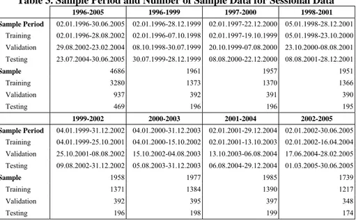
After such partition rule (70% - 20% - 10%) was applied, the investigation periods and the number of the samples for training, cross validation and testing data sets were organised as presented in Table 2 and Table 3 for daily and sessional data sets respectively.
Table 3. Sample Period and Number of Sample Data for Sessional Data
1996-2005 1996-1999 1997-2000 1998-2001 Sample Period 02.01.1996-30.06.2005 02.01.1996-28.12.1999 02.01.1997-22.12.2000 05.01.1998-28.12.2001 Training 02.01.1996-28.08.2002 02.01.1996-07.10.1998 02.01.1997-19.10.1999 05.01.1998-23.10.2000 Validation 29.08.2002-23.02.2004 08.10.1998-30.07.1999 20.10.1999-07.08.2000 23.10.2000-08.08.2001 Testing 23.07.2004-30.06.2005 30.07.1999-28.12.1999 08.08.2000-22.12.2000 08.08.2001-28.12.2001 Sample 4686 1961 1957 1951 Training 3280 1373 1370 1366 Validation 937 392 391 390 Testing 469 196 196 195 1999-2002 2000-2003 2001-2004 2002-2005 Sample Period 04.01.1999-31.12.2002 04.01.2000-31.12.2003 02.01.2001-29.12.2004 02.01.2002-30.06.2005 Training 04.01.1999-25.10.2001 04.01.2000-15.10.2002 02.01.2001-13.10.2003 02.01.2002-16.04.2004 Validation 25.10.2001-08.08.2002 15.10.2002-04.08.2003 13.10.2003-06.08.2004 17.06.2004-28.02.2005 Testing 09.08.2002-31.12.2002 05.08.2003-31.12.2003 06.08.2004-29.12.2004 01.03.2005-30.06.2005 Sample 1958 1977 1985 1739 Training 1371 1384 1390 1217 Validation 392 395 397 348 Testing 196 198 199 174
During analysis, the sizes for training, validation and testing data sets were kept fixed as 70%, 20% and 10%, in order to compare the performances for each model. However, fixing the percentages raised small mismatches between the daily and sessional data. For example, for the period 1996-1999, the testing data started on 02.08.1999 for daily data, however, it started on 30.07.1999 for sessional data. Although, a few similar mismatches could be observed, such mismatches in the sample period would not distort the results of the analysis.
3.2. Methodology
This study utilised three-layer (one hidden layer) multilayer perceptron models (feedforward neural network models), as these models are mathematically proved to be universal approximator for any function. According to Hornik et al. (1989), Cybenko (1989) and Hornik et al. (1990) three layered feedforward neural network models with nonlinear function in the hidden layers could approximate any continuos function well if there was sufficient hidden nodes in the hidden layer. Three different multilayer perceptron models were trained with different architectures. The first architecture had 7 processing elements (will be denoted as PE-7) in the hidden layer, the second one had 14 processing elements in the hidden layer (will be denoted as PE-14), and the third one had 28 processing elements in the hidden layer (will be denoted as PE-28).
Figure 1. Multilayer Perceptron Model
Figure 1 illustrates the basic model used in this study. The input layer composed of N units of xi (i = 1,2….N) and the hidden layer composed of R processing entities of
km (m = 1,2,…..R), and hence one output layer was vd. The output for the model
could be presented in the functional form as:
f R m N i i im mdg w x w g y ⎥ ⎥ ⎦ ⎤ ⎢ ⎢ ⎣ ⎡ ⎟ ⎟ ⎠ ⎞ ⎜ ⎜ ⎝ ⎛ =
∑
∑
=0 =0 ˆ (2)where, wim was the connection weights between input units and hidden processing
units, wmd was the connection weights between hidden processing units and the
output unit, g(.) and g(.)f were the activation functions for hidden processing
elements and output unit respectively.
………... x1 x2 x3 xi k1 k2 km vd ………. Input Layer Hidden Layer Output Layer
In the study the activation functions, g(.) and g(.)f, for hidden and output layers were
hyperbolic tangent and linear functions respectively. Equation 3 presents the activation functions mathematically:
x x g e e e e (x) g(x) f x x -x x = + − = = − ) ( tanh (3)
In order to optimise the neural network model defined above, the scaled conjugate gradient algorithm was utilised. The advantage of the scaled conjugate gradient was its ability to avoid the line search procedure, which was necessary for other conjugate methods.
Total of 12 multilayer perceptron models were trained to examine their effectiveness in forecasting ISE-100 index returns. In order to present the effectiveness of multilayer perceptron models in daily forecasts, 6 models were developed. The architectures of these models were 14-7-1, 14-14-1, 14-28-1 before sensitivity analysis and 10-7-1, 10-14-1, 10-28-1 after sensitivity analysis (the first, second and third numbers were representing the number of units in input layer, hidden layer and output layer respectively). Also, additional 6 models were developed to present the effectiveness of multilayer perceptron models in sessional forecasts of ISE-100 index. The architectures of the models used in sessional analysis were identical to daily analysis
3.3. Sensitivity Analysis
In the case of the neural network models, if the number of input variables is lower then the required level then the forecasting performance of the model can be limited. On the other hand if the number of input variables is higher than the required level again the forecasting performance of the model can be limited.In order to increase the forecasting accuracy, the most important variables should be included in the analysis.
The sensitivity analysis is important in determining the importance of the input variables for forecasting accuracy. The least important variables can be omitted from the data set in order to improve the forecast results (Kilimasauskas, 1994).
In this study the relative importance of each input variable was analysed by the use of sensitivity analysis. As a result of the sensitivity analysis 4 input variables were found to be least important. Theses input variables were 3 days and 5 days moving average for index (raw data), 3 days and 5 days moving average for volume (raw data). As a consequence, the neural network models were retrained with the remaining 10 input variables.
3.4. Performance Measure
Although there have been many different statistical methods existing in literature, the most common methods are sum of squared errors (SSE), mean absolute error (MAE), mean squared error (MSE), root mean squared error (RMSE), and mean absolute percentage error (MAPE).
However, the basic objective of the forecasting efforts is to beat the market, or in other words, gaining more returns than the average market return (Refenes, 1995). The statistical performance measures are providing a clue about the performance of the neural network models, but do not guarantee the profitability of the forecasts (Yao, et al., 1999).
Thus, in this study the profitability of the neural network models was analysed by the use of simple trading strategy. The trading strategy was:
⎩ ⎨ ⎧ < > = + Sell y If Buy y If Strategy Trading t t ; 0 , ; 0 , 1 (4) Where, yt was denoting the forecasted index return for trading period t. The
profitability of each model then is compared to market return for each investment period. In the case of calculating trading profits the transaction costs were ignored. (For the interested readers, the findings for the statistical performance measures are also provided in appendix).
4. Empirical Findings
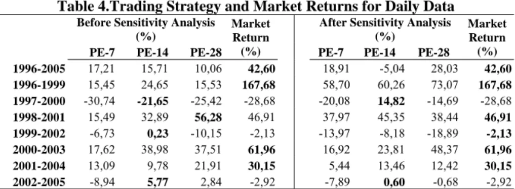
The results presented in this section were the findings for the testing period (out-of-sample data) of whole and sub-period data sets. As stated in the previous section, the testing period for each period was composed of the last 10% of data in the sample. Table 4 presents the returns generated by the training strategy, which are guided by the neural network models, and market return for the daily data.
Table 4.Trading Strategy and Market Returns for Daily Data
Before Sensitivity Analysis (%)
Market Return (%)
After Sensitivity Analysis (%)
Market Return (%)
PE-7 PE-14 PE-28 PE-7 PE-14 PE-28
1996-2005 17,21 15,71 10,06 42,60 18,91 -5,04 28,03 42,60 1996-1999 15,45 24,65 15,53 167,68 58,70 60,26 73,07 167,68 1997-2000 -30,74 -21,65 -25,42 -28,68 -20,08 14,82 -14,69 -28,68 1998-2001 15,49 32,89 56,28 46,91 37,97 45,35 38,44 46,91 1999-2002 -6,73 0,23 -10,15 -2,13 -13,97 -8,18 -18,89 -2,13 2000-2003 17,62 38,98 37,51 61,96 16,92 23,81 48,37 61,96 2001-2004 13,09 9,78 21,91 30,15 5,44 13,46 12,42 30,15 2002-2005 -8,94 5,77 2,84 -2,92 -7,89 0,60 -0,68 -2,92
*Bold characters denote highest return for the period
From the let-hand side of the table (returns before the sensitivity analysis), the trading strategy guided by neural network models could not generate satisfactory returns over the market return. For the all periods when the market return was positive, the neural network models could not beat the market except for the period of 1998-2001. On the other hand, in the case of negative market returns, the trading strategy could generate positive returns except for the period of 1997-2000. However, for the 1997-2000 period, the market return was –28.68%, the trading strategy was effective in limiting the loss at -21.65%.
The PE-14 model was the best model for the daily analysis before sensitivity analysis as it generated higher returns over the market for 3 periods (1997-2000,
1999-2002, 2002-2005). The PE-28 model could only beat the market and other models in 1998-2001. On the other hand, the PE-7 model could not beat the market in any of the periods.
The right hand side of the Table 4 presents the returns generated by the neural network models after sensitivity analysis. One could conclude that the sensitivity analysis had no use as the neural network models performances were worsen after the sensitivity analysis. At first glance, such reasoning could be accepted. Because the neural network models could beat the market in only two of the sub-periods, while it was 4 before sensitivity analysis. However, if the findings of the daily analysis before and after sensitivity were compared on the basis of average returns generated by each model, it could be observed that the sensitivity analysis increased returns generated by each model on average. However, such increases were not sufficient to beat the market.
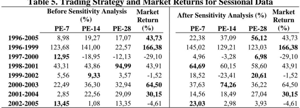
The returns generated by each of the neural network model for sessional data before and after the sensitivity analysis were reported in Table 5. The left-hand side of the Table 5 presented the return generated the neural network models prior to sensitivity analysis for the sessional data. It was observed that in four of the periods the neural network models could beat the market. These periods were 1997-2000, 1998-2001, 1999-2002 and 2002-2005. Interestingly, the same result was also reported for the daily analysis. However, this time the PE-7 model could beat the market in two of the periods (1997-2000, 2002-2005), while this model had no use in daily analysis. Furthermore, the PE-14 and PE-28 could only beat the market in 1999-2002 and 1998-2001 respectively.
Table 5. Trading Strategy and Market Returns for Sessional Data
Before Sensitivity Analysis (%)
Market Return (%)
After Sensitivity Analysis (%) Market Return (%)
PE-7 PE-14 PE-28 PE-7 PE-14 PE-28
1996-2005 8,98 19,27 17,07 43,73 22,38 37,09 56,12 43,73 1996-1999 123,68 141,00 22,57 166,38 145,02 129,21 123,03 166,38 1997-2000 12,95 -18,95 -12,13 -29,10 4,96 -3,28 6,98 -29,10 1998-2001 43,31 43,86 94,99 43,91 64,69 60,15 58,60 43,91 1999-2002 5,56 9,33 3,57 -1,52 18,52 -23,41 20,61 -1,52 2000-2003 22,49 36,30 32,94 64,50 37,63 74,26 36,22 64,50 2001-2004 2,85 22,56 29,09 30,15 14,56 18,49 27,04 30,15 2002-2005 13,45 1,08 13,35 -4,61 23,03 2,98 3,93 -4,61
*Bold characters denote highest return for the period
The right-hand side of the Table 5 presented the findings of the trading strategy after the sensitivity analysis. It was obvious that the sessional analysis with sensitivity increased the returns generated by neural network models. For 6 periods (out of 8) the neural network models could beat the market. In the case of market downtrends for the periods of 1997-2000, 1999-2002 and 2002-2005, the neural network models consistently beat the market with returns of 6,98%, 20,61% and 23.03%, respectively. However, during bull market the neural network models were able to beat the market for all the periods except for the periods of 1996-2000 and 2001-2004.
According to return calculations after sensitivity analysis, the PE-28 model was the best model during the periods of 1996-2005, 1997-2000 and 1999-2002. On the
other hand, PE-7 model is best during the periods 1998-2001 and 2002-2005. However, PE-14 model beat the others during the time interval of 2000-2003. When the findings of the study were interpreted as a whole, the results indicated that no model was superior to any other models in all of the periods. When the investment period changed, the performance of the neural network models was subject to change.
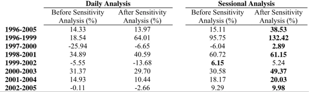
The effects of data frequency (daily and sessional) and sensitivity analysis (in terms of input variables) on the forecast performances of neural network models could be interpreted by the use of Table 6.
Table 6. Average Returns Generated by Daily and Sessional Analysis
Daily Analysis Sessional Analysis
Before Sensitivity Analysis (%) After Sensitivity Analysis (%) Before Sensitivity Analysis (%) After Sensitivity Analysis (%) 1996-2005 14.33 13.97 15.11 38.53 1996-1999 18.54 64.01 95.75 132.42 1997-2000 -25.94 -6.65 -6.04 2.89 1998-2001 34.89 40.59 60.72 61.15 1999-2002 -5.55 -13.68 6.15 5.24 2000-2003 31.37 29.70 30.58 49.37 2001-2004 14.93 10.44 18.17 20.03 2002-2005 -0.11 -2.66 9.29 9.98
*Bold characters denote highest return for the period
Table 6 was showing the average rate of return (simple average of returns generated by each model for each period) generated by each neural network model for each period for daily and sessional analysis before and after the sensitivity analysis. From the table its was clear that the profitability was directly effected from the data frequency. The profitability of neural network models greatly increased when the sessional data was used. In none of the periods, the forecasts of daily analysis could beat the sessional analysis according to average returns.
The effect of sensitivity analysis for the daily data was not clear. Although, the returns generated by neural network models were increased on average after sensitivity analysis, such increase was not satisfactory to conclude about the usefulness of the sensitivity analysis. However, in the case of the sessional analysis, the profitability of the neural network models after sensitivity analysis was greatly improved. The return generated by the neural network models after sensitivity analysis was higher for all periods except 1999-2002.
5. Conclusion
This study has been designed to forecast the daily and sessional returns for IMKB 100 index by the use of neural network models. In this manner, multilayer perceptron neural network models are trained and the forecasting effectiveness of the neural network models with and without sensitivity analysis is evaluated by the use of financial performance measure.
The remarkable findings of the study, is that (consistent with the literature) the performance of neural network models is time depended. No neural network model can consistently be superior to other models in all one of the investigation periods.
The data frequency and input selection are the other factors affecting the forecast performances of neural network models. Decreasing the data frequency (from daily to sessional data) increases the forecasting performance for ISE-100 index. The forecasts of sessional analysis are superior to the daily analysis in all the periods. Moreover, omitting the least important variables from the analysis by the use of sensitivity analysis has a positive impact on the forecasting performance of the neural network models.
Although, the findings of the study presented show promising results for the neural network models, in order to increase the efficiency of neural network models, further emphasis should be placed on the network architecture and input variables included.
References
ADYA, M. & COLLOPY, F. (1998). How effective are neural networks at forecasting and prediction? A review and evaluation. Journal of Forecasting, 17, pp. 487-495.
AKTAŞ, R., DOĞANAY, M. & YILDIZ, B. (2003). Mali başarısızlığın öngörülmesi: istatistiksel yöntemler ve yapay sinir ağı karşılaştırması, Ankara
Üniversitesi SBF Dergisi, 58(4), pp. 1-25.
ALTAY, E. & SATMAN, M.H. (2005). Stock market forecasting: Artificial neural networks and linear regression comparison in an emerging market. Journal of Financial Management and Analysis, 18(2), pp. 18-33.
BENLİ, Y.K. (2005). Bankalarda mali başarısızlığın öngörülmesi lojistik regresyon ve yapay sinir ağı karşılaştırması. Gazi Üniversitesi Endüstriyel Sanatlar Eğitim Fakültesi Dergisi, 16, pp. 31-46
BOYACIOĞLU, M.A., KARA, Y. (2006) Türk bankacılık sektöründe finansal güç derecelerinin tahmininde yapay sinir ağları ve çok değişkenli istatistiksel analiz tekniklerinin performanslarının karşılaştırılması. 10. Ulusal Finans Sempozyumu, 01-04 Kasım 2006, İzmir.
BROWNSTONE, D. (1996). Using percentage accuracy to measure neural network predictions in stock market movements. Neurocomputing, 10, pp. 237-250. CHANDRA, N. & REEB, D.M. (1999). Neural Networks in a Market Efficiency
Context. American Business Review, January, pp. 39-44.
CYBENKO, G. (1989). Approximation by superpositions of a sigmoidal function. Mathematics of Control, Signal and Systems, 2, pp. 303-314.
DARRAT, A.F. & ZHONG, M. (2000). On testing the random -walk hypothesis: A model comparison approach. The Financial Review, 35, pp. 105-124.
DEBOECK, G.J. & CADER, M. (1994). Pre- and post-processing of financial data. In: Trading on the Edge: Neural, Genetic, and Fuzzy Systems for Chaotic Financial Markets, Deboeck, G.J. (Ed.), John Wiley & Sons Inc.,pp. 27-45. DİLER, A.İ. (2003). İMKB Ulusal-100 endeksinin yönünün yapay sinir ağları hata
geriye yayma yöntemi ile tahmin edilmesi, İMKB Dergisi, 25-26, pp. 65-81 EGELI, B., ÖZTURAN, M., & BADUR, B. (2003). Stock market prediction using
artificial neural networks. Proceedings of the 3rd Hawaii International Conference on Business, Hawai, USA.
FADLALLA, A. & LIN, C.H. (2001). An analysis of the applications of neural networks in finance. Interfaces, 31, pp. 112-122.
GATELY, E. (1996). Neural Networks for Financial Forecasting, John Wiley & Sons, Inc.
GENCAY, R. (1996). Non-linear prediction of security returns with moving average rules. Journal of Forecasting, 15, pp. 165-174.
________. (1998). Optimisation of technical trading strategies and the profitability in the stock markets. Economic Letters, 59, pp. 249-254.
________.& STENGOS, T. (1998). Moving average rules, volume and the predicability of stock returns with feedforward networks, Journal of Forecasting, 17, pp. 401-141.
GÜNEŞ, H. & SALTOĞLU, B. (1998). İMKB getiri volatilitesinin makroekonomik konjonktür bağlamında irdelenmesi. Istanbul Stock Exchange Publilication. HORNIK, K., STINCHCOMBE, M. & WHITE, H. (1989). Multilayer feedforeward
networks are universal approximators. Neural Networks, 2, pp. 359-366.
________. (1990). Universal approximation of an unknown mappings and its derivatives using multilayer feedforward neural networks. Neural Networks, 3, pp. 551-560.
JANG, G. & LAI, F. (1994). Intelligent Trading of an Emerging Market. In: Trading on The Edge, Deboeck, G.J.(Ed.), John Wiley & Sons Inc., pp. 80-101.
Istanbul Stock Exchange, Evaluation and Statistics Department (2005). Factbook 2005. Avaliable from: http://www.imkb.gov.tr/veri.htm [Last accessed January 20, 2006],
KAASTRA, I. & BOYD, M. (1996). Designing a neural network for forecasting financial and economic time series. Neurocomputing, 10, pp. 215-236.
KAMIJO, K. & TANIGAWA, T. (1990). Stock price pattern recognition: a recurrent neural network approach. Proceedings of the IEEE International Joint Conference on Neural Networks, pp. 215-221.
KARAATLI, M., GÜNGÖR, İ., DEMİR, Y. & KALAYCI, Ş. (2005). Hisse senedi fiyat hareketlerinin yapay sinir ağları yöntemi ile tahmin edilmesi. Balıkesir Üniversitesi İİBF Dergisi, 2(1), pp. 22-48.
KILIMASAUSKAS, C.,C. (1994). Neural Network Techniques, In: Trading on the Edge, Deboeck, G.J. (Ed.), John Wiley&Sons, Inc., pp. 1-26.
KIM, S.H. & CHUNG, S.H. (1998). Graded forecasting using array of bipolar predictions: application of probabilistic neural networks to a stock market index. International Journal of Forecasting, 14, pp. 323-337.
KIMOTO, T., ASAKAWA, K., YODA, M. & TAJEOKA, M. (1990). Stock market prediction system with modular neural networks. Proceedings of the IEEE International Joint Conference, on Neural Networks, pp. 1-16.
KOHARA, K, ISHIKAWA, T., FUKUHARA, Y. & NAKAMURA, Y. (1997). Stock price prediction using prior knowledge and neural networks. Intelligent Systems in Accounting, Finance and Management, 6, pp. 11-22.
KRYZANOWSKI, L., GALLER, M. & WRIGHT, D., W. (1993). Using artificial neural networks to pick stocks. Financial Analysts Journal, 49/4, pp. 21-27. LAM, M. (2004). Neural Network techniques for financial performance prediction:
integrating fundamental and technical analysis. Decision Support Systems, 37, pp. 565-581.
MAASOUMI, E. & RACINE, J. (2002). Entropy and predicability of stock market returns, Journal of Econometrics, 107, pp.291-312.
OLSON, D. & MOSSMAN, C. (2002). Neural network forecasts of Canadian stock returns using accounting ratios. International Journal of Forecasting, 1, 2002, pp.1-13.
OZCAM, M. (1997). An Analysis Of The Macroeconomic Factors That Determine The Stock Returns.Capital Market Board Of Turkey Publication, No.75.
PHUA, P.K.H., MING, D. & LIN, W. (2001). Neural network with genetically evolved algorithms for stock prediction. Asia-Pacific Journal of Operational Research, 18, pp. 103-107.
REFENES, A.P. (1995). Testing Strategies and Metrics. In: Neural Networks in the Capital Markets, Refenes, A.P. (Ed.), , John Wiley & Sons, Inc., pp. 67-76. RODRIGUEZ, F.F., MARTEL, C., G. & RIVERO, S.S. (2000). On the profitability
of technical trading rules based on artificial neural networks: evidence from Madrid stock market. Economic Letters, 69, pp. 89-94.
RODRIGUEZ, J.V., TORRA, S. & FELIX, J.A. (2005). STAR and ANN models: Forecasting performance on Spanish Ibex-35 stock index. Journal of Empirical Finance, 12/3, pp. 490-509.
SAAD, E.W., PROKHOROV, D.V. & WUNSCH, D.C. (1998). Comparative study of stock trend prediction using time delay, recurrent and probabilistic neural networks. IEEE Transactions on Neural Networks, 9/6, pp. 1456-1470.
SINGH, S. (1999). A Long memory pattern modelling and recognition system for financial time-series forecasting. Pattern Analysis and Applications, 2, pp. 264-273.
STANSELL, S.R. & EAKINS, S.G. (2003). Forecasting the direction of change in sector stock indexes: An application of neural networks. Journal of Asset Management, 5/1, pp. 37-48.
SUN, Y.F., LIANG, Y.C., ZHANG, W.L., LEE, H.P., LIN, W.Z. & CAO, L.J. (2005). Optimal partition algorithm of the RBF neural network and its application to financial time series forecasting. Neural Computation & Application, 14, pp. 36–44
THAWORNWONG, S. & ENKE, D. (2003). Forecasting Stock Returns with Artificial Neural Networks. In: Neural Networks in Business Forecasting, Zhang, P.G. (Ed.), Idea Group Inc., pp.47-74.
VELLIDO, A., LISBOA, P.J.G. & VAUGHAN, J. (1999). Neural networks in business: A survey of applications (1992-1998). Expert Systems with Applications, 17, pp. 51-70.
WALCZAK, S. (2001). An empirical analysis of data requirements for financial forecasting with neural networks. Journal of Management Information Systems, 17/4, pp. 203-222.
WHITE, H. (1988). Economic prediction using neural networks: The case of IBM daily stock returns. Proceedings of the IEEE International Conference on Neural Networks, pp. 451-458.
WONG, F.S., WANG, P.Z., GOH, T.H. & QUEK, B.K., (1992). Fuzzy neural systems for stock selection. Financial Analysts Journal, 48, pp. 47-52.
YAO, J., TAN, C.L. & POH, H.L. (1999). Neural networks for technical analysis: A study on KLCI. International Journal of Theoretical and Applied Finance, 2/2, pp. 221-241.
YAO, J.T. & TAN, C.L. (2001). Guidelines for Financial Forecasting with Neural Networks. Proceedings of International Conference on Neural Information Processing, Shanghai China, 14-18 November, pp. 1-6.
YILDIZ, B. (2001). Finansal başarısızlığın öngörülmesinde yapay sinir ağı kullanımı ve halka açık şirketlerde ampirik bir uygulama. İMKB Dergisi, 17, pp. 51-67
YODA. M, (1994). Predicting the Tokyo Stock Market. In: Trading on The Edge, Deboeck, G.J. (Ed.), John Wiley & Sons Inc., pp. 66-79.
YÜMLÜ, S., GÜRGEN S.F. & OKAY, N. (2003). Financial time series prediction using mixture of experts, Lecture Notes in Computer Science, 2869, pp.553-560.
________. (2004). Turkish stock market analysis using mixture of experts, Engineering in Intelligent Systems (EIS 2004), Conference Proceedings.
________. (2005). A comparison of global, recurrent and smoothed-piecewise neural models for Istanbul Stock Exchange (ISE) prediction", Pattern Recognition Letters, 26(13), pp.2093-2103.
APPENDIX - Statistical Performances for Daily Data
Performance 1996-2005 1996-1999 1997-2000 1998-2001 1999-2002 2000-2003 2001-2004 2002-2005 Be fo re Se nsit ivit y Analysis PE-7
Mean Square Error 0,000259 0,002171 0,001917 0,000922 0,000928 0,000574 0,000250 0,000379 Normalised MSE 1,026183 1,743463 1,041960 1,060271 1,029747 1,259474 1,101355 1,258946 Mean Absolute Error 0,012963 0,032962 0,030679 0,023673 0,023329 0,018379 0,012424 0,015222
PE-14
Mean Square Error 0,000287 0,001813 0,001717 0,000928 0,000966 0,000572 0,000340 0,000304
Normalised MSE 1,138541 1,456096 0,933571 1,067251 1,072695 1,253870 1,492832 1,010774
Mean Absolute Error 0,013722 0,029281 0,028524 0,025071 0,023237 0,018497 0,014672 0,013778 PE-28
Mean Square Error 0,000346 0,002886 0,002025 0,000845 0,001138 0,000510 0,000251 0,000327 Normalised MSE 1,373548 2,317241 1,101043 0,971361 1,263738 1,119936 1,104112 1,087986 Mean Absolute Error 0,015436 0,039014 0,031998 0,022909 0,024492 0,017543 0,012634 0,014159
Af te r Se nsit ivit y Analysis PE-7
Mean Square Error 0,000263 0,001392 0,001980 0,000904 0,001037 0,000511 0,000258 0,000334 Normalised MSE 1,042809 1,118117 1,076487 1,039428 1,150954 1,121141 1,134382 1,111360 Mean Absolute Error 0,013141 0,025503 0,029857 0,023599 0,023690 0,017002 0,012896 0,014600
PE-14
Mean Square Error 0,000291 0,001386 0,001894 0,000885 0,001021 0,000508 0,000249 0,000316
Normalised MSE 1,153965 1,112698 1,029849 1,017995 1,133321 1,114161 1,096134 1,051255
Mean Absolute Error 0,013901 0,026180 0,029314 0,023498 0,023817 0,017210 0,012772 0,013994
PE-28
Mean Square Error 0,000256 0,001435 0,001951 0,000925 0,001122 0,000462 0,000247 0,000346 Normalised MSE 1,014034 1,152077 1,060821 1,064194 1,245578 1,014155 1,083908 1,151090 Mean Absolute Error 0,012760 0,025585 0,029921 0,023997 0,024641 0,016777 0,012549 0,013963
Bold characters indicate the best results for the year.
APPENDIX - Statistical Performances for Sessional Data
Performance 1996-2005 1996-1999 1997-2000 1998-2001 1999-2002 2000-2003 2001-2004 2002-2005 Be fo re Se nsit ivit y Analysis PE-7
Mean Square Error 0,0001178 0,0004470 0,0008122 0,0004953 0,0004056 0,0003216 0,0001306 0,0001325 Normalised MSE 1,0831949 0,9797059 0,9975259 1,0012437 1,0041581 1,3260049 1,2503449 1,0214192 Mean Absolute Error 0,0084086 0,0150171 0,0198808 0,0165128 0,0145872 0,0126587 0,0087935 0,0085583
PE-14
Mean Square Error 0,0001248 0,0006864 0,0008320 0,0005045 0,0004054 0,0002673 0,0001192 0,0001369 Normalised MSE 1,1469797 1,5046324 1,0218306 1,0199540 1,0037011 1,1023720 1,1414471 1,0558462 Mean Absolute Error 0,0087213 0,0184726 0,0201513 0,0166322 0,0147348 0,0113942 0,0084280 0,0084680
PE-28
Mean Square Error 0,0001363 0,0007867 0,0009119 0,0004925 0,0004403 0,0003201 0,0001157 0,0001307
Normalised MSE 1,2534041 1,7244861 1,1199019 0,9956549 1,0901658 1,3198289 1,1075516 1,0073477
Mean Absolute Error 0,0090191 0,0193776 0,0209144 0,0169618 0,0154787 0,0131183 0,0081735 0,0083046
Af te r Se nsit ivit y Analysis PE-7
Mean Square Error 0,0001085 0,0004559 0,0007682 0,0004519 0,0004023 0,0002513 0,0001115 0,0001285
Normalised MSE 0,9974266 0,9993611 0,9433928 0,9135795 0,9960458 1,0364256 1,0671836 0,9908466
Mean Absolute Error 0,0080089 0,0150226 0,0198270 0,0161265 0,0147095 0,0110019 0,0080995 0,0084736
PE-14
Mean Square Error 0,0001092 0,0004629 0,0007940 0,0004628 0,0004187 0,0002454 0,0001094 0,0001330 Normalised MSE 1,0039517 1,0146507 0,9751152 0,9356988 1,0366826 1,0120116 1,0469358 1,0255191 Mean Absolute Error 0,0080292 0,0150783 0,0197789 0,0164136 0,0147817 0,0109601 0,0080618 0,0084133 PE-28
Mean Square Error 0,0001072 0,0004492 0,0007999 0,0004754 0,0004023 0,0002608 0,0001072 0,0001371 Normalised MSE 0,9853684 0,9846622 0,9823196 0,9612002 0,9959873 1,0753852 1,0263557 1,0571179 Mean Absolute Error 0,0079857 0,0148974 0,0196159 0,0164677 0,0146627 0,0113312 0,0079908 0,0086717