*Corresponding author. Tel.:#32-16-32-25-66; fax:# 32-16-32-29-86.
E-mail address:[email protected] (L. Gelders).
The (R,
Q) inventory policy subject to a compound Poisson
demand pattern
Peter Matheus, Ludo Gelders*
K.U. Leuven}Centre for Industrial Management, Celestijnenlaan 300 A, 3001 Heverlee, Belgium Received 26 March 1998; accepted 13 September 1999
Abstract
Most inventory management models are based upon rather restrictive assumptions, e.g. unit sized demands and the normal distribution for total demand during replenishment time. In a majority of inventory management systems, circumstances seem to allow these simpli"cations, and inventory policies based upon these assumptions yield satisfying results. However, in some particular cases, these simpli"cations di!er fundamentally from the actual conditions and particle. Therefore, application of the models mentioned above can result in an overinvestment in inventory or in an unacceptable low service level. One of the situations in which we cannot rely on these simpli"ed inventory models is studied in this paper. We consider an inventory subject to a probabilistic non-unit sized demand pattern, and we propose an exact and an approximate reorder point calculation method for the (R,Q) inventory policy. The exact algorithm involves formulas for the discrete distributions of the total demand during replenishment time and the undershoot. The approximate method is based on the use of continuous distributions, and will be more appropriate when historical data are sparse. Results of both approaches are compared. The algorithms proposed in this study are simple, fast and easy to implement in a variety of (existing) inventory management systems. ( 2000 Elsevier Science B.V. All rights reserved.
Keywords: Inventory management; (R,Q) inventory policy; Reorder point calculation method
1. Introduction
The situation studied in this paper is a very familiar one in inventory management: we consider a central stock with orders arriving from a variety of customers (Fig. 1). The customer order size is not "xed, but follows a discrete probability distribu-tion. The central stock could be anything, from a central inventory of spare parts in a chemical plant to a supermarket.
Normally, this kind of inventory is managed by an order point and order up to level system, the (s,S) policy (e.g. [1,2]). In general, this policy o!ers the best way to deal with large demands crossing the reorder point s, causing substantial under-shoots. However, in some circumstances, the inven-tory manager has to use"xed reorder quantitiesQ, e.g. if the supplier uses standard packings contain-ing a"xed number of units, or if the`supplierais a internal production process with a "xed lotsize. In this case the inventory may be managed by a (R, Q) policy, which will be determined in this paper.
We propose calculation methods for the reorder pointRof a (R, Q) inventory policy with a target
Fig. 1.
service level, subject to an non-unit sized demand pattern. The reorder quantity is known (e.g. the EOQ or a"xed quantity determined by other con-siderations). The demand pattern is compound Poisson. This means that demand arrivals consti-tute a Poisson process (the interarrival times are exponentially distributed), and that the individual demand size follows some unspeci"ed discrete dis-tribution. The Poisson assumption is appropriate if the customer population consists of a large group of individuals acting independently. Furthermore, we assume the leadtime ¸ between supplier and inventory to be"xed. In case of stockouts backlog-ging is applied, and the inventory level is continu-ously monitored.
The service levelb, used in this study, is de"ned as the steady-state percentage of the total number of units requested met directly from stock on hand. Assume that a cycle is the time elapsed between two consecutive moments at which a replenishment or-der is received. Then the following basic formula may be used for the calculation ofb, though stan-dard theory of regenerative processes cannot be applied [2]:
b"1!E(demand that goes short in one cycle)
E(total demand in one cycle)
(1)
withEdenoting the expected (or average) value of the expression between brackets.
As the backordering situation is considered in this study, the average demand per cycle equals the average amount received per cycle. Thus,
E(total demand in one cycle)"Q. Let us de"ne following quantities:
B
1"Ecycle),(shortage present at the beginning of a
B
2"E(shortage at the end of a cycle). This means that B
1 is the expected shortage just after a replenishment order has been received and
B
2is the expected shortage just prior to the arrival of a replenishment order. Thus,
b"1!(B2!B1)
Q . (2)
With ubeing the stochastic quantity representing the undershoot (the amount by which the reorder point is crossed when the reordering is triggered), andd
L being the stochastic quantity representing
the leadtime demand, it is clear that
B
1"E([u#dL!R!Q]`), (3)
B
An exact algorithm for the computation ofB
1and
B
2(based on a discrete stochastic model and tested by means of simulation), and an approximate method (based on a continuous stochastic model) will be proposed. Results obtained by both methods will be compared for some testcases.
2. The discrete model
The basic problem in developing closed expres-sions forB
1andB2is to"nd the discrete probabil-ity distributions for the undershoot u and the demand during leadtimed
L.
For the calculation of the distribution of d
L,
Adelson's recursion scheme [3], can be applied. Let jbe the arrival rate of the demands,¸the ("xed) leadtime, andUi the probability of receiving a de-mand of sizei(i"1, 2,2,m, withmthe maximum
size). The probability r
0 of having zero demands during the leadtime is given by
r
0"exp(!j¸). (5)
The probability r
k of having a total leadtime
de-mand ofkunits can be obtained by the following recursive formula:
This recursion scheme o!ers an e$cient and nu-merically stable calculation method.
For the determination of the undershoot distri-bution, we use the formula proposed by Karlin [4] and Silver et al. [5]. Let E(d) denote the average demand size, thenm
k, the probability of having an
undershoot of k units during stock cycle, can be calculated by:
Though this formula was proposed as an approxi-mation of the undershoot distribution in an inven-tory controlled by a (s, S) policy, we proved it to be exact in the case of the (R, Q) policy (Appendix A).
Now that closed expressions for the discrete dis-tributions ofd
Landuare available, only one
prob-lem remains to be solved: in formulas (3) and (4) a summation of the two stochastic quantities
d
Landuappears. This means one needs the
convo-lution of these two distributions. Therefore we cal-culatef
k, the probability that the summation of the
undershoot and the total demand during leadtime in a stockcycle equalsk:
f
For reasons that become clear later, one only has to calculate this distribution for values ofkfrom 0 to
R#Q.
Now it is clear that
B
some algebra leads to
b"R`Q+
The procedure described above, resulting in this simple formula, o!ers a calculation method for the service levelbfor a given reorder pointR.
The exactness of this algorithm was tested by means of a discrete event simulation [6]. The following assumptions were made:
j"1,
¸"5 (except for the`outliersacase, then¸"2),
Q"200.
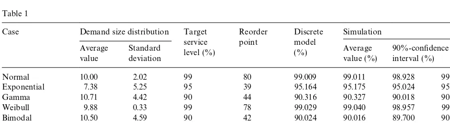
Table 1
Case Demand size distribution Target service
Normal 10.00 2.02 99 80 99.009 99.011 98.928 99.094
Exponential 7.38 5.25 95 39 95.164 95.175 95.024 95.326
Gamma 10.71 4.42 90 44 90.316 90.327 90.018 90.636
Weibull 9.88 0.33 99 78 99.029 99.040 98.957 99.123
Bimodal 10.50 4.59 90 42 90.024 90.016 89.700 90.332
Random 11.77 5.05 99 102 99.026 99.031 98.922 99.139
Outliers 19.00 27.15 95 106 95.073 95.063 94.727 95.398
The distributions were generated as follows: in four cases, we took a well-known continuous prob-ability distribution (normal, exponential, gamma and Weibull). They were truncated at 0.5 and 20.5, normalized and discretized. For two other cases, the `bimodala and the `outliersa, a normalized superposition of the probability density functions of two normal distributions was used (representing two types of customers). In the `bimodala case these distributions were rather close to each other (the two types of customers have only a slightly di!erent average demand size). In the `outliersa case there was a big gap between both distributions (two very di!erent types of customers). The result-ing distribution again was truncated (the ` bi-modalaat 0.5 and 20.5, the `outliersa at 0.5 and 105.5), normalized and discretized. In the`randoma case, a sequence of 20 normalized random numbers was generated, representing the probability of hav-ing a demand size of 1}20 units.
After the determination of these discrete distribu-tions, we calculated (in an enumerative way) the reorder point R, required to attain the predeter-mined target service levelb.
Since the reorder point must be integer, the actual service level always was a bit higher than the target value. Afterwards these results were tested by means of a discrete simulation program. For every case 30 simulation runs were performed (except for the `normala case where we used 173 runs), and every run consisted of 4000 stock cycles. An average service level and a con"dence interval (90%) were calculated. As one can see in Table 1, the results obtained by application of the algorithm proposed above, fall very well
within the (narrow) limits of these con"dence intervals.
The results from three simulations con"rm that the calculation method described above is exact. Furthermore, this algorithm is simple, straightfor-ward and numerically stable.
However, even though the formulas are easy to program, the implementation of this inventory con-trol model in new or existing stock management systems could cause some problems. The manage-ment of data, the necessary input for the algorithm, could be fairly complex. The inventory manage-ment software needs support and input from a database containing the arrival rate j, the leadtime¸, the reorder quantityQ, and the discrete order size distributions for all the products in the inventory under consideration. This database should be updated with every transactions, and as demand sizes may vary considerably, such a database could be very memory consuming.
So, though the model proposed above could be very useful for critical items, or items with rather compact order size distributions, or simply (be-cause of its exactness) for benchmark calculations in tests for approximate algorithms, we should try to "nd a good approximate model with less data requirements. In the next section an approximation based upon a continuous stochastic model is pro-posed.
3. The continuous model
probability distributions. Therefore, we build an approximate continuous model, using approximate continuous probability distributions. For reasons that will become clear, the normal and the gamma distributions are applied. For these distributions, one only has to store the average value and the standard deviation. This study is based on results obtained by Tijms [2] for an inventory under peri-odic review, managed by a (s,S) policy.
Again closed expressions forB
1andB2have to be developed. This means one has to"nd the distri-bution of the summation of the undershootuand the total leadtime demandd
L.
Assume thatkis the average demand size,pis the standard deviation of demand size, and D
L is the
stochastic quantity denoting the summation of to-tal leadtime demand,d
L, and the size of the demand
that triggers the reordering-decision. Letf(x) be the approximated continuous probability density func-tion (pdf) ofu#d
L,g(x) the pdf ofdL andh(x) the
pdf ofD
L. Then one can easily prove by extension
of results obtained by Tijms [2] that
f(x)+1
k(P(dL)x)!P(DL)x)), x*0 (12) (withPdenoting the probability of the logical ex-pression between brackets), and assuming that the pdf of the demand size has a"nite third moment:
P
= withCsome constant positive real number (C*0).Thus, The only remaining problem is the calculation of the de"nite integrals. By a proper choice of the distributionsg(x) andh(x), this turns out to be an easy task. In this study the normal distribution and the gamma distribution (for which the integrals become incomplete gamma integrals) are used. In both cases fast codes are widely available. The parameters of both approximate distributions re-main to be determined. This can be done by match-ing of the"rst two moments, the average value and the standard deviation. Thus,g(x) is de"ned by
This approximate algorithm was tested for several cases.
Again discrete demand size distributions were generated in the same way as in the previous sec-tion, and for these distributionspandk were cal-culated. The following assumptions were made:
j"1,
¸"5 (except for the`outliersacase, then¸"2),
Q"200.
With the exact discrete algorithm, the reorder point
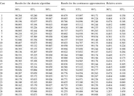
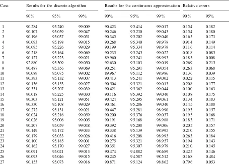
distribution, the relative error lies between a min-imum of 0.017% and a maxmin-imum of 2.204% and reaches an average value of 0.393%. The worst results were obtained in the `outliersa case. The gamma approximation seems to yield better results: the relative error lies between 0.001% and 0.769% with an average value of 0.145%. Again the worst cases can be found among the `outliersa. The in-ferior performance of the Normal approximation may be due to the`tailaof this distribution in the negative domain.
In general, the results are satisfying and cer-tainly su$cient for most practical purposes. Therefore this algorithm, based on a continuous stochastic model, forms an interesting alternative for the exact, but memory consuming, discrete algorithm.
4. Conclusion
In this paper an exact and e$cient algorithm is proposed for the reorder point calculation of an inventory managed by an (R,Q) policy, subject to a compound Poisson demand. This algorithm is based upon Adelson's recursion scheme [3] and an undershoot distribution formula that was proved to be correct. Though the algorithm could easily be implemented in a new or existing inventory man-agement system, the data requirements could pose some practical problems. So, when dealing with very critical items, or in cases where vast demand size data are available, or simply when an exact benchmark calculation is needed, this discrete model yields a simple and fast solution.
Whenever historical data are nor present and the inventory manager can only give a rough estima-tion of the form of the demand size distribuestima-tion (the average value and the standard deviation), or whenever one cannot dispose of a su$ciently large database, the approximate continuous model, pro-posed in the last section of this paper, can be applied. This model is an extension of results ob-tained by Tijms [2] for the periodic review (s, S) policy. It is based upon an approximation of the discrete distributions with normal or gamma prob-ability density functions. Results from a variety of tests clearly indicate that the performance of this
continuous model is su$cient for most practical situations.
Appendix A
Theorem. In a continuously monitored inventory,
controlled by a (R, Q) policy and subject to a com-pound Poisson demand pattern, the probabilitym
u of
having in a stock cycle an undershoot of u units equals:
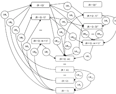
Proof. The inventory is modelled as a continuous
Markov chain (see Fig. 2).
In this chain three types of states are de"ned:
(z) forz"R#1 toR#Q!m,
(z)@and (z)Aforz"R#Q!m#1 toR#Q
withzdenoting the stock position. So every stock position betweenR#1 andR#Q!mde"nes one state, the stock positions between R#Q!m#1 and R#Q de"ne two separate states. The di! er-ence between the states (z)@ and (z)A will become clear later. The steady-state probabilities are p(z),
p((z)@) andp((z)A).
The transitions in this chain are de"ned by stock movements. Two types of stock movements are considered. The"rst type is caused by the arrival of a demand that does not cross the reorder point. This means that the original stock position is lowered by the demand size. The second type is caused by a demand that crosses the reorder point
R, and thus increases the stock position with the reorder quantityQminus the demand size.
Fig. 2.
splitting of a Poisson stream (under probabilities
U1,U2,2,Um) generatesm new Poisson streams
with parameters Uij(i"1, 2,2,m). These
para-meters Uij de"ne the transition rates in the con-tinuous Markov chain (see Fig. 2).
Now the di!erence between the states (z)@and (z)A can be explained.
A state (z)@can only be reached by a stock move-ment of the second kind (thus with a reordering decision). If the original stock position was x, the sizedof the demand causing the transition must be equal to or larger thanx!R. The resulting state is (z)@, with
z"x#Q!d. (A.2)
Whenever state (z)@is entered, an undershoot of size
uoccurs, with
u"d!(x!R)"Q#R!z. (A.3)
Because of the PASTA property of Poisson processes (Poisson arrivals see time average),
p((z)@) not only equals the fraction of time that the system remains in state (z)@, but also equals the probability that a stock movement enters this state, and thus results in an undershoot of size u. Therefore, the probability that a stock movement causes an undershoot of size u equals
p((Q#R!u)@).
On the other hand, a state (z)Acan only be the result of stock movement of the "rst kind. This means that (z)Acan only be reached from a state (x)@ or (x)Aifxis strictly larger thanz.
The probability that a demand causes a reorder-ing-decision equals
R`Q
+
j/R`Q~m`1
Table 2
Overview of testables and reorder points
Case Order size distribution Reorder point for target service level
Based upon Average
value
Standard deviation
90% 95% 99%
1 Normal 10.00 2.02 38 54 80
2 Normal 10.01 3.00 38 54 82
3 Normal 10.05 3.82 39 55 84
4 Normal 10.35 5.39 42 60 90
5 Exponential 8.86 5.63 33 50 78
6 Exponential 7.38 5.25 24 39 65
7 Exponential 5.14 4.16 10 23 43
8 Exponential 2.54 1.97 0 5 17
9 Gamma 4.10 2.78 4 15 31
10 Gamma 5.92 3.89 14 27 48
11 Gamma 7.87 3.76 26 40 64
12 Gamma 10.71 4.42 44 61 91
13 Weibull 9.18 2.12 33 48 73
14 Weibull 9.51 1.18 34 50 75
15 Weibull 9.73 0.65 36 51 77
16 Weibull 9.88 0.33 37 52 78
17 Bimodal 10.32 5.10 42 59 89
18 Bimodal 10.50 4.59 42 60 90
19 Bimodal 10.32 4.77 41 58 88
20 Bimodal 10.50 5.14 43 60 91
21 Random 10.63 5.46 44 62 93
22 Random 11.77 5.05 51 69 102
23 Random 10.32 5.61 42 60 90
24 Random 10.60 5.66 44 62 93
25 Outliers 55.00 45.05 216 271 383
26 Outliers 37.00 41.32 152 198 294
27 Outliers 19.00 27.15 73 106 180
28 Outliers 10.91 9.44 12 29 77
Fig. 3.
Now, one can compute the conditional probability m
uthat a demand that triggered a reordering causes
an undershoot of sizeu:
m
u"
p((R#Q!u)@)
+R`Qj/R`Q~m`1p((j)@), u"0, 1, 2,2,m!1. (A.4)
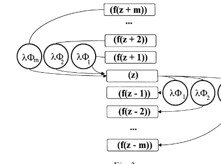
The only problem that remains to be solved is the computation of the steady-state probabilitiesp((z)@). Let us de"ne a reduced continuous Markov chain. In this chain the states (z)@and (z)Aare com-bined into one state (z) (forz"R#Q!m#1 to
R#Q). The rest of the chain remains unchanged. Let p
Table 3
Results of the normal approximation
Case Results for the discrete algorithm Results for the continuous approximation Relative errors
90% 95% 99% 90% 95% 99% 90% 95% 99%
1 90.284 95.240 99.009 89.879 95.097 99.171 0.449 0.150 0.164
2 90.107 95.059 99.047 89.685 94.909 99.224 0.468 0.158 0.180
3 90.196 95.037 99.051 89.766 94.896 99.244 0.476 0.148 0.196
4 90.093 95.198 99.015 89.649 95.112 99.244 0.492 0.090 0.231
5 90.093 95.226 99.029 89.624 95.100 99.255 0.523 0.132 0.229
6 90.095 95.164 99.069 89.737 94.973 99.283 0.533 0.201 0.216
7 90.218 95.233 99.021 89.692 94.938 99.191 0.483 0.310 0.171
8 90.127 95.309 99.050 92.600 94.974 99.034 0.301 0.351 0.017
9 92.880 95.356 99.069 90.157 95.019 99.146 0.365 0.354 0.077
10 90.487 95.075 99.002 89.653 94.787 99.155 0.484 0.303 0.154
11 90.089 95.132 99.007 89.950 94.919 99.176 0.491 0.224 0.170
12 90.393 95.153 99.027 89.894 95.058 99.244 0.467 0.100 0.219
13 90.136 95.207 99.039 89.922 95.032 99.187 0.452 0.284 0.150
14 90.331 95.225 99.030 89.164 95.060 99.174 0.449 0.173 0.145
15 90.018 95.121 99.051 89.909 94.954 99.196 0.436 0.175 0.146
16 90.303 95.108 99.029 89.938 94.945 99.176 0.434 0.171 0.148
17 90.272 95.131 99.021 89.838 95.032 99.244 0.481 0.105 0.225
18 90.024 95.216 99.059 89.588 95.122 99.273 0.485 0.099 0.216
19 90.026 95.006 99.005 89.582 94.892 99.277 0.493 0.120 0.225
20 90.207 95.059 99.048 89.776 94.954 99.263 0.478 0.110 0.217
21 90.149 95.172 99.033 89.713 95.096 99.267 0.484 0.080 0.236
22 90.179 95.033 99.026 89.771 94.971 99.258 0.453 0.065 0.235
23 90.100 95.185 99.001 89.655 95.100 99.233 0.494 0.089 0.234
24 90.162 95.170 99.027 89.725 95.091 99.258 0.484 0.082 0.233
25 90.091 95.021 99.013 90.794 96.312 99.688 0.780 1.359 0.681
26 90.093 95.046 99.015 91.253 96.604 99.764 1.287 1.639 0.757
27 90.153 95.073 99.016 91.975 97.168 99.908 2.021 2.204 0.900
28 90.052 95.208 99.016 89.289 95.141 99.933 0.847 0.070 0.926
reduced chain. Then it is clear that
p
r(z)"p(z), z"R#1,2,R#Q!m, (A.5)
p
r(z)"p((z)@)#p((z)A)
z"R#Q!m#1,2,R#Q. (A.6)
The functionf(x) is de"ned by
f(x)"
G
x ifR#1)x)R#Q,
x!Q ifx'R#Q,
x#Q ifx(R#1.
(A.7)
Fig. 3 shows only a part of the reduced continuous Markov chain, namely those states that are connec-ted with state (z) (for z"R#1 to R#Q). This
reduced chain clearly constitutes a closed loop, with the following set of steady-state equations:
m
+
j/1 jUjp
3(f(z#j))"p3(z)
m
+
j/1 jUj
forz"R#1,2,R#Q,
R`Q+ z/R`1
p
3(z)"1. (A.8)
The structure of this set of equations clearly implies that the steady-state probabilities of all these
Qstates must be equal, thus,
p
3(z)"
1
Table 4
Results of gamma approximation
Case Results for the discrete algorithm Results for the continuous approximation Relative errors
90% 95% 99% 90% 95% 99% 90% 95% 99%
1 90.284 95.240 99.009 90.423 95.414 99.017 0.154 0.182 0.008
2 90.107 95.059 99.047 90.246 95.230 99.045 0.154 0.180 0.001
3 90.196 95.037 99.051 90.345 95.202 99.040 0.165 0.173 0.011
4 90.093 95.198 99.015 90.268 95.340 98.978 0.914 0.149 0.038
5 90.095 95.226 99.029 90.199 95.334 98.979 0.116 0.114 0.050
6 90.218 95.164 99.069 90.235 95.245 99.022 0.018 0.085 0.047
7 90.127 95.223 99.021 89.960 95.241 98.993 0.185 0.008 0.028
8 92.880 95.309 99.050 92.630 95.103 99.019 0.269 0.215 0.032
9 90.487 95.356 99.069 90.251 95.291 99.054 0.263 0.068 0.016
10 90.089 95.075 99.002 89.967 95.112 98.986 0.136 0.039 0.016
11 90.393 95.132 99.007 90.413 95.241 99.002 0.022 0.115 0.006
12 90.136 95.153 99.027 90.504 95.321 99.013 0.208 0.177 0.014
13 90.331 95.207 99.039 90.421 95.362 99.044 0.100 0.163 0.005
14 90.018 95.225 99.030 90.116 95.392 99.040 0.108 0.175 0.010
15 90.303 95.121 99.051 90.424 95.295 99.061 0.134 0.183 0.010
16 90.330 95.108 99.029 90.461 95.286 99.040 0.145 0.188 0.011
17 90.272 95.131 99.021 90.447 95.281 98.990 0.193 0.157 0.031
18 90.024 95.216 99.059 90.200 95.376 99.037 0.195 0.168 0.023
19 90.026 95.006 99.005 90.191 95.168 98.988 0.183 0.171 0.017
20 90.207 95.059 99.048 90.392 95.208 99.006 0.205 0.157 0.042
21 90.149 95.172 99.033 90.338 95.139 98.995 0.210 0.155 0.038
22 90.179 95.033 99.026 90.416 95.208 98.995 0.263 0.184 0.031
23 90.100 95.185 99.001 90.275 95.321 98.957 0.194 0.143 0.044
24 90.162 95.170 99.027 90.351 95.307 98.979 0.210 0.145 0.049
25 90.091 95.021 99.013 90.474 94.882 98.689 0.425 0.146 0.328
26 90.093 95.046 99.015 90.245 94.587 98.512 0.168 0.484 0.508
27 90.153 95.073 99.016 90.871 95.124 98.862 0.796 0.053 0.155
28 90.052 95.208 99.016 89.968 95.413 99.691 0.093 0.215 0.682
This means that the inventory positionzat steady state is uniformly distributed on the integers [R#1;R#Q]. The same result was obtained in a recent study of AxsaKter [7].
Now, the steady-state probabilities of the states (R#Q!u)@ in the original continuous Markov chain can be calculated by solving next equation (foru"0, 1,2,m!1):
Some algebra yields the following result:
p((R#Q!u)@)"1
the reorder quantityQ, though it can be extended to cases for whichmis larger thanQ.
Appendix B
For the overview of testcases and reorder points see Table 2.
For the results of the normal approximation see Table 3.
For the results of the gamma approximation see Table 4.
References
[1] R.H. Hollier, K.L. Mak, C.L. Lam, An inventory model for items with demands satis"ed from stock or by special de-liveries, International Journal of Production Economics 42 (1995) 229}236.
[2] H.C. Tijms, Stochastic Models, an Algorithmic Approach, Wiley, Chichester, 1995.
[3] R.M. Adelson, Compound poisson distribution, Operations Research Quarterly 17 (1996) 73}75.
[4] S. Karlin, The application of renewal theory to the study of inventory policies, in: K. Arrow, S. Karlin, H. Scarf (Eds.), Studies in the Mathematical Theory of Inventory and Pro-duction, Stanford University Press, Stanford, CA, 1958. [5] E.A. Silver, D.F. Pyke, R. Peterson, Inventory Management
and Production Planning and Scheduling, 3rd Edition, Wiley, New York, 1998.
[6] A.M. Law, W.D. Kelton, Simulation Modeling and Analy-sis, 2nd Edition, McGraw-Hill, New York, 1991. [7] S. AxsaKter, Simple evaluation of echelon stock (R,Q)