*Corresponding author. Protek Computer Systems Inc., Perpa Ticaret Merkezi, Elektrokent, Kat 13, No 1981, Okmeydani, 80270 Istanbul, Turkey. Tel:.#90 (212) 210-1730; fax:#90 (212) 210-1765.
E-mail: [email protected] (H. Polatoglu)
Optimal procurement policies under price-dependent demand
Hakan Polatoglu
!
,
*, Izzet Sahin
"
!Frank Sawyer School of Management, Suwolk University, Boston, MA 02108, USA "School of Business Administration, University of Wisconsin-Milwaukee, Milwaukee, WI 53201, USA
Received 19 June 1998; accepted 17 September 1998
Abstract
We study a periodic-review inventory model where, in addition to the procurement quantity, price is also a decision variable. We develop a model where demand in each period is a random variable having a price- and, possibly, period-dependent probability distribution, with the expected demand decreasing in price. The model includes price limits
and"xed ordering costs in addition to unit procurement holding and shortage costs. We study the optimal policies which
jointly maximize the discounted expected pro"t over a"nite planning horizon. We characterize the form of the optimal procurement policy under a general price}demand relationship and give a su$cient condition for it to be (s
n,Sn) type. We
also discuss some special cases and extensions to the basic model, including the in"nite horizon problem. ( 2000 Elsevier Science B.V. All rights reserved.
Keywords: Pricing; Inventory; (s,S) policy
Notation
n period index (n"1 corresponds to the last period)
N total number of periods in the planning horizon
i
n beginning inventory level before ordering in periodn
q
n beginning inventory level after ordering in periodn
p
n price in periodn
Pl price#oor
P
6 price ceiling
c unit procurement cost
r unit shortage cost
h unit holding cost
v unit salvage value at the end of the planning horizon
K
n "xed ordering cost in periodn
a periodic discount factor
X(p) random demand when price isp
XM (p) expected demand as a function of price ("E[X(p)])
¸(p) lower bound on random demand, 0)¸(p))X(p) ;(p) upper bound on random demand,X(p));(p)(R f(x;p) probability density function ofX(p)
F(x;p) probability distribution ofX(p)
p
n(qn) optimal price when the inventory level isqn in periodn
M
n(in,pn,qn) ncost)-period (periodsn}1) pseudo-pro"t function (pro"t excluding the e!ect of the"xed ordering
MM n(i
n,pn,qn) expected value ofMn(in,pn,qn)
MM w
n(in,qn) MnM-period expected pseudo pro"t when the optimal value ofw pnis implemented in periodn, i.e., n(in, qn),MM n(in,pn(qn),qn)
PM (i
n, pn) n-period expected pro"t when the optimal value ofqnis implemented in periodn
PM w(i
n) n-period expected pro"t when the optimal values ofqnandpnare implemented in periodn
d(z) Heavyside function,d(z)"0 forz)0 andd(z)"1 forz'0 [z]` positive value function, [z]`"zd(z)
1. Introduction
Under increased competition, inventory-based businesses are forced to better coordinate their procure-ment and marketing decisions, to avoid carrying excessive stock when sales are low or shortages when they are high. An e!ective means of such coordination is to conduct the inventory control and pricing decisions jointly. The main task in doing so is to determine the optimal inventory policy, given the price}demand relationship that is expected to prevail in the market place in the short term.
In addressing the above issue, we are concerned in this paper with a single-item, periodic-review inventory system where the vendor, who enjoys a degree of monopoly power in the market place, is in a position to in#uence demand by its pricing decisions. It is thus confronted with simultaneous pricing and procurement quantity decisions, which would jointly maximize the present value of expected pro"t over a planning horizon. We will assume that the ordering policy does not change the demand pattern during the planning horizon.
Ordering cost, shortage cost and temporal increases in the procurement cost are among the important factors that force the decision maker to carry inventories. Holding cost has the opposite e!ect. Thus, in the absence of pricing, the main decision problem is to determine the optimal inventory levels to strike a balance between these opposing factors, under a given demand forecast, cost structure, and a set of operating conditions.
There are critical di!erences between a"xed-price, periodic-review inventory model [1] and a model that also includes pricing decisions. The economical interpretations of these di!erences relate to the various ways that price plays into the decision problem. First, price is a decision variable that determines the revenue per unit sold. Second, price is a factor that in#uences the demand, thus the period-ending inventory levels. In addition, when backlogging occurs, apart from the amount of backorders, the backlogging policy must also account for the price that applies to backorders and the timing of revenue collection. For instance, backorders could be sold at the current price in advance, or at a future price set at the time of delivery.
Therefore, when the decision maker confronts the pricing and inventory decisions simultaneously, in addition to the two opposing cost-related e!ects that we noted above, price-related factors must also be taken into account. Mainly, there will be a trade-o!between the high-price low-demand and low-price high-demand scenarios, in terms of discounted total revenue. This revenue trade-o!, however, will not be
independent of the above described cost trade-o!, since the demand levels (i.e., inventory levels) will be a!ected by the pricing decisions. Unfortunately, this complex relationship between the cost and revenue trade-o!s does not allow the model to simplify into separate pricing and procurement decisions.
Various versions of the procurement-and-pricing model has been studied in the literature. In his pioneer-ing work, Whitin [2] proposed a link between price theory and inventory control. He noted that such a model would have stronger managerial implications, as compared to"xed-price models. Later, Mills [3,4] and Karlin and Carr [5] established a conceptual framework for a general inventory model, where price is a decision variable. Subsequent studies concentrated mostly on the characterization of the optimal solution for some special cases of the general model [6}13]. Thomas [14] provided some numerical examples to demonstrate the nature of the decision problem under the presence of"xed ordering costs. More recently, Gallego and Van Ryzin [15] studied the continuous-time version of the problem, and Petruzzi [16] investigated the approximate solutions under a learning approach. Also, under a dynamic model with Bayesian learning about the demand distribution, Subrahmanyan and Shoemaker [17] studied a number of numerical examples which provide insights about the sensitivity of optimal prices and inventory levels to changes in the unit procurement cost, price elasticity of demand, form of the demand distribution and the expected demand function.
The existing analytical models impose rather restrictive assumptions on the form of the expected demand function (e.g., concavity assumptions in [9,11,12]), demand distribution (e.g., multiplicative demand in [9], additive demand in [9,11]), or the cost structure (e.g., parameter restrictions and no"xed ordering cost in [11,10]) in analyzing the optimal procurement policy. In this paper, by relaxing some of the more limiting modeling assumptions, we seek to characterize the fundamental properties of the optimal procurement policy and the resulting expected pro"t in a more general setting (i.e., general demand distribution, linear cost structure with the addition of set-up cost). We also address the sensitivity of the optimal procurement policy to the underlying price-dependent demand uncertainty.
In what follows, we describe the price}demand relationship in Section 2, develop the basic model in Section 3, and characterize its solution in Section 4. The rest of the paper is devoted to special cases and extensions. We consider the in"nite-horizon problem in Section 5, the model with no"xed ordering costs in Section 6, the non-stationary extensions of the basic model in Section 7, and the special case with determinis-tic demand in Section 8. Section 9 is devoted to some concluding remarks. Sections 4 and 5 include numerical examples. Proofs are given in the appendix.
2. Demand uncertainty
It has been a common practice in demand modeling to express random demand as a combination of an expected demand function, which exhibits some form of price-dependency, and a random term, which is price-independent. This approach conveniently isolates the e!ects of price and uncertainty, while retaining mathematical tractibility. However, it has some shortcomings.
Under theadditive model[3,5,9,11], we haveX(p)"XM (p)#ewhereXM (p) is a decreasing function ofpand e is a random variable with E[e]"0. The additive model can also be interpreted as a homoscedastic regression model whereXM (p) represents the regression function andeis the error term. One implication of this model is that while the expected demand is a function of the price, the demand variance is price-independent (demand distribution shifts as price varies). Also, the model allows for negative demand, unless the price values are bounded from above.
In addition to these, there are models that represent random demand by a mixture of additive and multiplicative terms [10,12,13], such as X(p)"XM (p)a
1(e)#a2(e), or X(p)"a1(p)#ea2(p), where a1 and
a
2are di!erentiable functions.
Additional simpli"cation can be achieved by assuming that the price}demand relationship is perfectly predictable. This leads to thedeterministic model,X(p)"XM (p), which serves as a"rst-order approximation, and which has been utilized as a benchmark in the literature [3,5,9,12]. It has been reported in these studies that the form of demand uncertainty, whether it is additive or multiplicative, plays a critical role in determining optimal prices. Optimal prices are lower than their deterministic counterparts under the additive demand model, while they are found to be greater under the multiplicative demand model. Additional "ndings about the form of demand uncertainty, as it impacts optimal prices and inventory levels, are reported in [18] p. 617.
In this study, we represent the demand by a continuous random variable, distributed over the range [¸(p),;(p)] with a known density functionf(x;p).¸and;are di!erentiable functions which represent the bounds on demand, where 0)¸(p))X(p));(p)(Rfor allp. For convenience, we"rst assume station-arity, whereby the demand density is given byfin all periods. We then show in Section 8 that the results we obtain for the "nite-horizon problem can be extended to non-stationary (period-dependent) demand distributions.
There is empirical evidence that consumers react to price in purchasing. Other things being equal, a lower price facilitates demand in a`fairamarket. Therefore, it is natural to assume that the probability that demand is less than a given levelx,F(x;p)"P[X(p))x], is a non-decreasing function of price. That is,
LF(x;p)
Lp *0 ∀x3(¸(p),;(p)). (1)
It follows from Eq. (1) that F(x;p
1))F(x;p2) for p1(p2. Thus, price induces a stochastic ordering of
demand distributions.
The expected demand is given by
XM (p)"
U(p)
P
L(p)
xf(x;p) dx"
=
P
0
[1!F(x; p)] dx. (2)
It also follows from Eqs. (1) and (2) thatXM (p) is a decreasing function ofp:
LF(x;p)
Lp *0N
dXM (p) dp "!
=
P
0
LF(x;p) Lp dx(0.
3. Mathematical model and assumptions
Consider a periodic-review inventory system withNperiods where the decision variables areq
nandpn. The
review periods are linked by period-ending inventory levels such that the leftovers are transferred fully to the next period and shortages are lost. That is,i
n"[qn`1!X(pn`1)]`for 0)n)N!1, andiN*0 is a given
parameter. At the beginning of a period, the vendor decides how much to order (q
n!in) and what price to
charge until the next decision point. There is a"xed cost of ordering (K), but no cost is assumed for pricing.
Therefore, it is for the vendor's bene"t to reconsider pricing at each decision epoch.
We assume that the vendor has full information about the inventory and procurement costs, and the demand distributions in all periods of the planning horizon. At the beginning of a review period, say periodn,
given the inventory position, the vendor is to determine the procurement quantity and the price to maximize the expectedn-period pro"t which represents the expected value of the sum of the current period's pro"t and the discounted optimal expected pro"t to be obtained during the remaining periods.
LetPnl and Pn
6be the price #oor and the price ceiling, respectively, in period n, such that the interval
[Pnl,Pn
6] represents the range of allowable prices. Then, the sequencesMP1l, P2l,2,PNlNandMP1
6, P26,2,PN6N
establish limiting-price pro"les during the planning horizon. In regulated markets, these pro"les represent the temporal rules of regulation. Also, in a case where a manufacturer might issue price limits for its dealers (price-maintenance), or provide`suggested retail pricesa, the allowable price ranges could be represented by the limiting-price pro"les.
In the basic model, without loss of generality, we assume uniform pro"les where the feasible price values in any period are betweenPlandP
6. If there is no price regulation or other constraint on prices, then the price
limits may be taken as 0 andp
=, respectively, wherep=, referred to as the`null priceain the literature, is the
highest possible price level at which there will be no demand, that is, P[X(p))0]"1 for all p*p
=.
Allowingp
="Rleads to detailed technical considerations (see [8,9]) which we choose to avoid in this paper.
We assume that inventory costs are proportional to period-ending inventory levels. The cost and discount-factor parameters may be allowed to change from period to period. However, as in the case of the demand distribution, we keep them time-invariant for convenience in developing the basic model (see Section 8 for non-stationary extensions of the basic model). We take P
6'c so that it is possible to make pro"t. In
addition, the leftovers at the end of the planning horizon are assumed to be salvaged at a discount price, that is,v)c.
Under these assumptions, then-period optimal expected pro"t, as a function ofi
n, is obtained from
PM w
n(in)"maxMPM n(in,pn): pn3[Pl,P6]N,
and
PM
n(in,pn)"maxMMM n(in,pn,qn)!Kd(qn!in):qn*inN,
whereMM nis the expected value of then-periodpseudo-pro,tfunction which is de"ned forn*1 as
M
n(in, pn,qn)"!c(qn!in)#
G
aPM w
n~1(0)#pnqn!r(X(pn)!qn), 0)qn)X(pn),
aPM w
n~1(qn!X(pn))#pnX(pn)!h(qn!X(pn)), X(pn))qn,
withPM w
0(i0)"v[i0]`. This leads to
MM n(i
n, pn,qn)"(pn#r!c)qn!rXM (pn)!(pn#r#h)H(pn,qn)#cin#aPM
w
n~1(0)[1!F(qn; pn)]
#a
qn~L(pn)
P
0
PM w
n~1(x)f(qn!x;pn) dx, (3)
whereH(p
n,qn)"E[[qn!X(pn)]`] is the expected value of leftovers at the end of periodn. It is seen that
H(p
n,qn) is a convex increasing function inqnand an increasing function inpn; its additional properties are
given in [19].
Therefore, the overall decision problem is described by
PM w
n(in)"maxMMM
w
n(in,qn)!Kd(qn!in):qn*inN (4)
MM w
n(in,qn)"maxMMM n(in,pn,qn):pn3[Pl,P6]N"MM n(in,pn(qn), qn), (5)
for alln*1, wherep
n(qn) represents the optimal price for a givenqnin periodn. The objective is to determine
the optimal decision variablespw
n and q
w
n for alln, which jointly maximizePM Nfor a giveniN. Note that if
PM w
4. Model solution
In order to determine the optimal procurement policy for periodn, we need to characterize the form of
MM w
n is additively separable ininandqn. Hence, it su$ces to characterize the form ofMM
w
n(0,qn). For that
purpose, we need to solve the maximization problem:
MM w
It turns out that the solution methods that have been developed for the"xed price (i.e.,Pl"P
6) versions of
the model [20}23] are not directly applicable for the solution of the problem at hand. Instead, we will follow a new solution approach which follows the inductive setting described in [21].
4.1. Form of the optimal procurement policy
The dynamic programming problem represented by Eq. (6) is worked out in the appendix. The results are summarized below in a theorem and a corollary after the following de"nitions.
De5nition.LetG(i,p,q)"(p#r!c)q!rXM (p)!(p#r#h!ac)H(p,q)#ci, andGw
Note that the generic functionGrepresents the expected pro"t in a single-period, lost-sales model where the unit salvage value is c(i.e., the leftovers are returned to the supplier at the original cost). It will play a critical role in the characterization ofMM w
n, and in establishing bounds on the optimal control parameters.
The following theorem describes the form ofMM w
n in general:
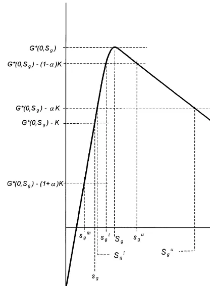
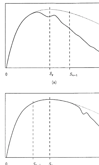
Theorem 1.¹here exist an even integer k
Fig. 1. De"nitions of the critical inventory levels underGw (0,q).
Corollary 1.For n*2,smg(s1
n, sknn~1(s
l
g, s6g(sknn,and S
l
g(Sn(S6g; also,if sg(s11, then sg(s1n.
Regarding the condition of unimodality of MM w
1(0,q1) in Theorem 1, there are analytical di$culties
in proving this property, except for some special cases [3,5,8,12,19,24]. For instance, it is reported in [19] that MM w
1(0,q1) is unimodal if (1) demand is deterministic, (2) demand is additive, e has a uniform
distribution and XM (p) is linear, or (3) demand is multiplicative, e has an exponential distribution and
XM (p) is linear. The discussions of unimodality and su$cient conditions can be found in the above-cited references.
SinceGis a special case of MM 1(with v"c), under the unimodality assumption,Gw
is also a unimodal function with a maximizer atS
gand a reorder point atsg((Sg). Thus, it follows from (a) and Corollary
1 (s1
n~1(Sg) that MM
w
n(0,qn) is an increasing function ofqn on [0,s1n~1]. Furthermore, (a) implies that the
optimal pricing decision,p
n(qn), forqn3[0,s1n~1] is given by argmaxMG(0,p,qn):p3[Pl, P6]N, the maximizing
price under the generic single-period model. (Note that ifq
n)s1n~1, there will be an order placed in period
n!1; hence, the inventory carried over to periodn!1 would worthac, and in this case the pricing decision is based only on G.)
It is implied by (b) and (c) thatMM w
n(0,qn) is bounded by two unimodal functions which are at mostaK
apart on [s1
n~1,sknn~1~1]. Hence, (b) and (c) establish bounds onMM
w
n(0,qn) based on the value of the optimal
(n!1)-period pro"t, provided that an order takes place in periodn!1. In this case, the contribution of the current period's pro"t is limited to betweenGw
(0,q
n) andG
w (0,q
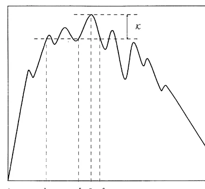
Fig. 2. A generaln-period expected pseudo-pro"t function,MM w
Thus, under the optimal solution, the increase in expectedn-period pro"t, upon raising the stock level from 0 toq
n, must be greater than or equal to the change in one-period expected pro"t (withv"c) under a similar
stock movement (i.e.,Gw (0,q
n)!G
w
(0, 0)). This increase, however, is limited byGw (0,q
n)!G
w
(0, 0)#aK. Property (b) extends the upper bound functionGw
(0,q
n)!aMM
w
n~1(0,s1n~1)#aK over [sknn~1~1,R). On the
other hand, it follows from (d) thatMM w
n(0,qn) isaK-decreasing ([22]) over [Sg,sknn~1~1], and the functional value
ofMM w
n, evaluated at any point beyondsknn~1~1, is strictly below the global maximum ofMM
w
n(0,Sn).
A general expectedn-period pseudo-pro"t function, as characterized by Theorem 1, is depicted in Fig. 2. It is seen that there could be more than one order-up-to level, and for each order-up-to level there could be more than one reorder interval. This characterization is weaker than that in the"xed-price model, where it can be shown that in each period a single optimal reorder-point, order-up-to-level policy exists [21].
The possible presence of multiple order-up-to levels poses serious di$culties in characterizing and computing the optimal procurement policies. These di$culties, however, can be circumvented if the beginning inventory level before ordering in an arbitrary periodnis less than or equal toskn
n. Then, since
MM w
n(0, 0) is"nite andMM
w
n(0,qn) tends to decline asqntends to in"nity, the optimal procurement policy can be
characterized as follows provided thati
n)sknn:
n, the `reorder regiona, is the union of reorder intervals, given by
[0,s1
n]X[s2n, s3n]X2X[sknn~2,sknn~1] andOMnis the complement ofOnwith respect to [0,sknn]. Note that under
the unimodality condition imposed onMM w
1, we havek1"2 andq
w
1 is determined by an (s1,S1) policy.
In implementing the above optimal procurement policy, we need to computeskn
n for each period, which can
be a computational burden. Instead, a stronger but more useful condition can be established by referring to Corollary 1, where we haves6
g)sknn. That is, we replace the condition of the above optimal policy (in)sknn) by
i
n)s6gwhich involves the computation ofs6gonce and in advance by using the problem primitives. Also, it is
seen that the conditioni
n)sknnis satis"ed ifSn(s6gfor allnandiN)SN.
The fundamental di!erence between the (s
n,Sn) policies de"ned for the"xed-price models [20,21] and the
policy we de"ne in Eq. (8) is that, at each decision epoch, the vendor has to make a pricing decision whether or not it decides to place an order. Thus, the vendor needs to determine the optimal price, p
n(in), at the
beginning of each review period, given the observed value ofi
n. This requires the preparation of price tables
for the vendor to read the optimal prices from. These tables can be prepared simultaneously during the computation of reorder points and the order-up-to level in each period.
4.2. A suzcient condition for a single reorder point
Properties (b) and (c) in Theorem 1 indicate thatMM w
n(0,qn) isaK-increasing over [s1n~1, s
l
g]. Theoretically,
this allows for more than one reorder point. However, operating a system under multiple reorder points could be a burden in practice. Determination of the critical levelss1
n,s2n,2, sknnfor all periods with su$cient
accuracy could be di$cult. It is, therefore, important to know under what conditions there exists a single reorder point (i.e.,k
n"2).
It follows from property (a) in Theorem 1 thatMM w
n(0,qn) is increasing over [0,s1n~1]; thus, ifs1n)s1n~1, that
is if MM w
n(0,s1n~1)*MM
w
n(0,Sn)!K, then kn"2 and s1n is the only reorder point. However, this is not
a convenient su$cient condition, since, under a general demand distribution, the value of s1
n~1, or
MM w
n(0,s1n~1), is not analytically measurable with su$cient accuracy.
Another possibility is to show thatMM w
n(0,qn) is increasing over [s1n~1, s
g], and investigate the su$cient conditions under which MM
w
gwith arbitraryqnandq@n. This leads to the following result:
Corollary 2.MM w
n(0,qn)is non-decreasing in qnover [s1n~1, s
l
g]for n*1,that is there exists a single reorder point
(k
The RHS in Eq. (9) is a concave increasing function ofp
n, andF(qn;pn) is assumed to be a non-decreasing
function ofp
nfor allqn(see Section 2).
In view of Eq. (9), we can make the following observations. If the vendor administers a higher price, he is able to increaseF(q
n;pn), the likelihood that there will be no shortage at levelqn, to a desired level, while the
relative weight of unit underage cost rises (relative weight of unit overage cost declines). Hence, the vendor is inclined to increase the stock level to aboveq
nand this continues until a break-even point is reached. This is
veri"ed by the fact thatLG(0,p,q)/Lq*0 under Eq. (9). Thus, based on the demand distribution and unit costs that prevail in the market, Eq. (9) re#ects the vendor's capability to increase the expected current period pro"t by increasing the stock level to abovesl
g. In other words, Eq. (9) attributes a higher monopoly power to
the vendor than the vendor would have in its absence. In this interpretation, we utilized the myopic notion that the higher the monopoly power, the less responsive is the demand to changes in price. That is, probability of satisfying the demand fully,F(q
n;pn), does not respond strongly to an increase in price, since
the increase inF(q
n; pn) is limited by the RHS in Eq. (9).
Under Theorem 1 and Corollary 2, the optimal procurement policy is de"ned by
qw
provided thati
n)s6gis satis"ed forn'1. It also follows thats
l
g)Snforn*1, such thats
l
gis a lower bound
on order-up-to levels.
Note that in order to havek
n"2,MM
w
n(0,qn) need not be increasing over [s1n~1,s
l
g]. There could be other
conditions leading to the same result. Our experience with a number of numerical examples suggests that cases withk
n'2 would be rare in practice.
4.3. Suzcient conditions for the optimality of (s
n, Sn)policies
If, in property (d), the range forq
nwere established as [Sg,R), thenMM
w
n(0,qn) would be characterized as
aK-decreasing function over [S
g,R),Snwould be the only order-up-to level, and there would be no need for
the conditioni
n)sknnin Eq. (8) or Eq. (10). This is precisely the case in the development of the optimality of
(s
n,Sn) policies under the "xed-price (Pl"P6) model [21].
In the following corollary, we investigate the su$cient conditions under whichMM w
n assumes a desirable
shape over [S
g,R) to yield a single order-up-to level.
Corollary 3.MM w
n(0,qn)*MM
w
n(0,q@n)!aKfor all qnand qn@ with Sg)qn(q@n,if s1)Sgand
(p
n#r#h!ac)F(qn;pn)*pn#r!c,∀pn3[Pl,P6],for n*1. (11)
Note that for largeqvalues,F(q;p) tends to 1 (particularly,F(q; p)"1 whenq*;(p)), and this complies well with condition Eq. (11). That is,MM w
n(0,qn) isK-decreasing in the limit asqntends to in"nity. Also, it is
intuitive that at considerably large inventory levels, the vendor would tend to reduce the price substantially, even below the unit procurement cost, in order to deplete inventories. In this regard, it is seen in Eq. (11) that the condition tends to hold when c and h get larger and r gets smaller (it holds at all q levels when
p#r!c)0)p#r#h!ac, that is, ac!h!r)p)c!r). In general, the condition tends to hold whencandhget larger orrgets smaller.
Thus, under Theorem 1 and Corollary 3, the optimal procurement policy is characterized by
qw
n"
G
S
n ifin3On,
i
n ifin3OMnorin'sknn.
Also, under both Corollaries 2 and 3, it follows from Theorem 1 thatk
n"2 for allnandq
w
n is determined by
an (s
n,Sn) policy:q
w
n"in#(Sn!in)d(s1n!in).
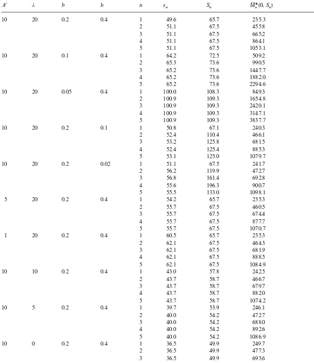
4.4. Numerical example
To demonstrate our "ndings, we consider a 5-period problem de"ned by the base parameter set
c"0.5,r"1.5,h"0.4,v"0.1,K"5,a"0.95; the expected demand functionXM (p)"ae~bpwitha"150 and b"0.2; the price limits Pl"0.1 and P
6"10; and the additive-uniform demand distribution F(x;p)"0.5(x!XM (p)#j)/jfor!j)x!XM (p))jwithj"20. (j"0 corresponds to the deterministic demand case.) For sensitivity analyses, we used multiple parameter values as h"0.02, 0.1, 0.4;
K"1, 5, 10;b"0.05, 0.1, 0.2; andj"0, 5, 10, 20.
Using a computer program, we computed the expected pseudo-pro"t functionsMM w
1,MM
w
2,2,MM
w
5over the
q
nrange of [0, 250] with a step size of 1. The resulting optimal values of the control parameters and the
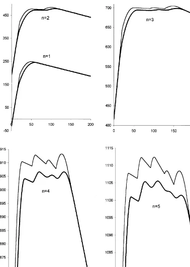
critical functional values are shown in Tables 1 and 2. Also, the pseudo-pro"t functions computed for j"0,K"10, the deterministic demand case, and j"10,K"10 are plotted in Figs. 3 and 4.
Table 1
Critical inventory levels, prices and pseudo-pro"t values under the 5-period example problem
K j b h n s
n Sn MM
w
n(0,Sn) pn(Sn)
10 20 0.2 0.4 1 49.6 65.7 235.3 5.5
2 51.1 67.5 455.8 5.5
3 51.1 67.5 665.2 5.5
4 51.1 67.5 864.1 5.5
5 51.1 67.5 1053.1 5.5
10 20 0.1 0.4 1 64.2 72.5 509.2 10.0
2 65.3 73.6 990.5 10.0
3 65.2 73.6 1447.7 10.0
4 65.2 73.6 1882.0 10.0
5 65.2 73.6 2294.6 10.0
10 20 0.05 0.4 1 100.0 108.3 849.3 10.0
2 100.9 109.3 1654.8 10.0
3 100.9 109.3 2420.1 10.0
4 100.9 109.3 3147.1 10.0
5 100.9 109.3 3837.7 10.0
10 20 0.2 0.1 1 50.8 67.1 240.3 5.5
2 52.4 110.4 466.1 5.5
3 53.2 125.8 681.5 5.5
4 52.4 125.4 885.3 5.5
5 53.1 125.0 1079.7 5.5
10 20 0.2 0.02 1 51.1 67.5 241.7 5.5
2 56.2 119.9 472.7 5.5
3 56.8 161.4 692.8 5.5
4 55.6 196.3 900.7 5.5
5 55.5 133.0 1098.1 5.5
5 20 0.2 0.4 1 54.2 65.7 235.3 5.5
2 55.7 67.5 460.5 5.5
3 55.7 67.5 674.4 5.5
4 55.7 67.5 877.7 5.5
5 55.7 67.5 1070.7 5.5
1 20 0.2 0.4 1 60.5 65.7 235.3 5.5
2 62.1 67.5 464.3 5.5
3 62.1 67.5 681.9 5.5
4 62.1 67.5 888.5 5.5
5 62.1 67.5 1084.9 5.5
10 10 0.2 0.4 1 43.0 57.8 242.5 5.6
2 43.7 58.7 466.7 5.5
3 43.7 58.7 679.7 5.5
4 43.7 58.7 882.0 5.5
5 43.7 58.7 1074.2 5.5
10 5 0.2 0.4 1 39.7 53.9 246.1 5.6
2 40.0 54.2 472.7 5.5
3 40.0 54.2 688.0 5.5
4 40.0 54.2 892.6 5.5
5 40.0 54.2 1086.9 5.5
10 0 0.2 0.4 1 36.5 49.9 249.7 5.5
2 36.5 49.9 477.3 5.5
3 36.5 49.9 693.6 5.5
4 36.5 49.9 899.1 5.5
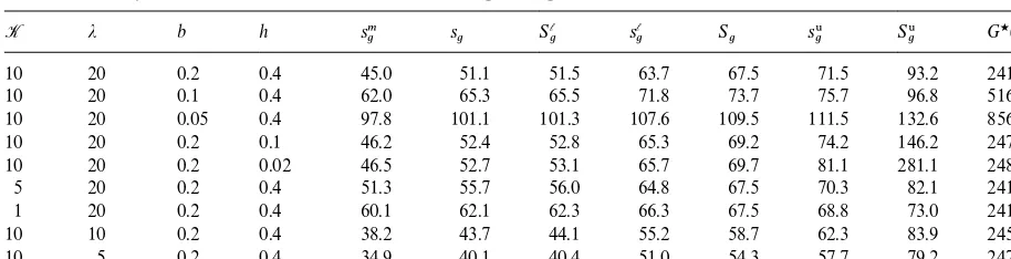
Table 2
Critical inventory levels that are obtained under the generic pseudo-pro"t function
K j b h smg s
g S
l
g s
l
g Sg s6g S6g G
w (0,S
g)
10 20 0.2 0.4 45.0 51.1 51.5 63.7 67.5 71.5 93.2 241.7
10 20 0.1 0.4 62.0 65.3 65.5 71.8 73.7 75.7 96.8 516.0
10 20 0.05 0.4 97.8 101.1 101.3 107.6 109.5 111.5 132.6 856.1
10 20 0.2 0.1 46.2 52.4 52.8 65.3 69.2 74.2 146.2 247.2
10 20 0.2 0.02 46.5 52.7 53.1 65.7 69.7 81.1 281.1 248.8
5 20 0.2 0.4 51.3 55.7 56.0 64.8 67.5 70.3 82.1 241.7
1 20 0.2 0.4 60.1 62.1 62.3 66.3 67.5 68.8 73.0 241.7
10 10 0.2 0.4 38.2 43.7 44.1 55.2 58.7 62.3 83.9 245.7
10 5 0.2 0.4 34.9 40.1 40.4 51.0 54.3 57.7 79.2 247.7
We observe that the optimal control values are quite sensitive to the price senstivity of demand (note that
bis the price elasticity multiplier of the expected demand). The more sensitive the expected demand to price, the less is the expected pro"t. As for the holding cost, smallerhvalues tend to yield considerably higher order-up-to levels.
Comparing the critical inventory levels listed in Tables 1 and 2, we see that the conditions given in Corollary 1 hold in each case. We also note thatS
n)s6gin all cases excepth"0.1 andh"0.02, for which the
reorder-region order-up-to level policy will be optimal.
Table 1 shows that the optimal prices evaluated at respective order-up-to levels are the same in all periods. Consequently, if an order is to be placed in each period, then the optimal prices in successive periods will be constant. We also observe that demand uncertainty has considerable impact on the parameters of the optimal procurement policy. As the demand variance is decreased (i.e.,jis decreased), the order-up-to and reorder levels both tend to be lower, and the vendor foresees higher expected pro"ts.
On the other hand, on comparing the deterministic and probabilistic pseudo-pro"t curves in Fig. 3, we "nd that the deterministic values are greater than the corresponding probabilistic values, especially, about theq
nmid-range, which includes respective order-up-to levels.
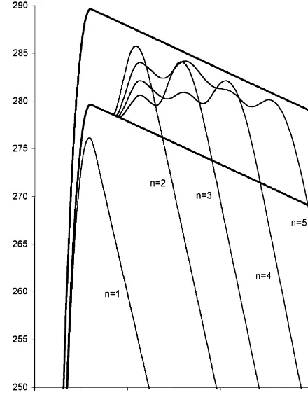
In Fig. 4, we plot MM w
n(0,qn)!MM
w
n(0, 0) vs. qn together with the boundary functions. It is seen that the
properties listed in Theorem 1 and Corollary 1 hold. The boundary functions established in Eq. (7) also satisfy the conditions (b@) and (c@). We also observe that the pseudo-pro"t curves exhibit considerable slope changes across theq
nmid-range.
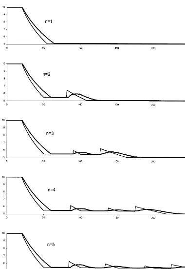
The best price trajectoriesp
n(qn), evaluated forn"1, 2,2, 5, are plotted in Fig. 5. The"gure shows that
the optimal pricing decision at a given inventory level is not necessarily trivial. We observe that p
n(qn) is
generally decreasing in q
n, but it can exhibit mild increases, or stagnate (become `stickya) over various
q
nranges where it does not respond to changes in stock levels. Also, on comparing the deterministic and
probabilistic optimal prices, we observe that it is not necessarily true that the deterministic prices are lower than the probabilistic prices or vice versa (cf. [4,5]).
Intuitively, price should be lower at higher stock levels, so as to facilitate higher demand to deplete the excess inventories. However, the vendor would still tend to increase the price for two basic reasons: to shrink the demand so that there will be leftovers for future periods, or to realize a higher pro"t per unit sold. If the "xed ordering cost in a future period is to be saved by satisfying that period's demand by carying a part of the current inventory forward, then both of these reasons will prevail. Once the total cost of inventory holding and the di!erential cost of procurement breaks even with the savings in the"xed ordering cost, however, it would not be pro"table to consider carrying stock into future periods. Asngets larger, there are more periods ahead to consider; thus, there could be a recurrence of this break-even behaviour at higherq
nlevels. This can
be seen in Fig. 5 by comparing p
5(q5) with p2(q2). The passage from one pricing regime to another, at
a break-even point, need not be smooth and there could be sudden changes inp
n(qn).
Fig. 3. Expected pseudo-pro"t curves, MM w
Fig. 4. Combined representation of the curves in Fig. 3. The thin curves representMM w
n(0,qn)!MM w
n(0, 0) vs.qnforn*1 and the thick curves represent the boundary functionsGw
(0,q
n)!G w
(0, 0) andGw (0,q
n)!G w
(0, 0)#K.
5. In5nite-horizon model
In this section, we study the in"nite-horizon version of the model. We drop the period indices from the notation and rewrite the expected pseudo-pro"t function from Eq. (6) as
MM w
(0,q)"max
G
G(0,p,q)#aMM w(0,s1)#a
q~L(p)
P
0
[MM w
(0,x)!MM w
(0,s1)]`f(q!x;p) dx:p3[Pl,P 6]
H
"G(0,p
q,q)#aMM
w
(0,s1)#a
q~L(pq)
P
0
[MM w
(0,x)!MM w
(0,s1)]`f(q!x;p
q) dx, (12)
wherep
q,p(q), the maximizing price atq.
The solution forMM w
(0,q) involves the integral in Eq. (12) which represents the convolution of the density function with a "ltering function based on MM w
(0,q) (i.e., the function MM w
(0,q) is "ltered over the level
MM w
(0,s1)). Because of this, we need to solve the integral Eq. (12) recursively. In each stage of the solution,
MM w
(0,q) is established over a non-overlapping interval, and the solution obtained is employed in the next stage.
It follows from Eq. (12) that for 0)q)s1 we have MM w
where the index in roman numeral denotes the stage number. Successive stages I, II, III,2correspond to
intervals [0,s1], [s1,s2],[s2,s3],2, respectively.
In the next stage, we haves1)q)s2for which the e!ective integration range starts ats1in Eq. (12) and we have
which is arenewal equation[25] with solution
MM w
however, then we need to consider theqrange beyonds2and pass to the next stage. Evaluating Eq. (12) fors2)q)s3, we obtain
IIinside the integral is obtained earlier, it can be substituted in the above to solve forMM
w
III.
The fourth stage will involve another renewal equation. Fors3)q)s4, we have
"G(0,p
q,q)#
a 1!aG
w
(0,s1)[1#F(q!s2; p
q)!F(q!s1; pq)!F(q!s3;pq)]
#a
s2
P
s1
MM w
II(0,x)f(q!x; pq) dx#a q~L(pq)
P
s3
MM w
IV(0,x)f(q!x;pq) dx,
which is a renewal equation onMM w
IV. The solution for this equation can be obtained by following a similar
procedure to the one used in solving forMM w
II(0,q).
Ifs4)s6g, then we stop. Otherwise, we follow the same solution process to establishMM w
in the next two stages, and check the stopping criterion.
This method works in principle. However, there is a computational di$culty due to the fact that critical inventory levels s1,s2,s3,2 are unknown in advance. They have to be computed simultaneously as we
establishMM w
numerically.
One approach is to start with the assumption thats1"s
g. Based on this initial value ofs1,MM
w can be established over [0,s2] and the value ofs2can be found by incrementing the value ofquntilMM w
II(0,q) equals
MM w
II(0,s1). Note thats2will be the "rst point greater than s1satisfying the above equality. Likewise, the
process can be continued to includes3ands4and so on. Once the stopping condition (s6
g)sk) is satis"ed,
using the current solution ofMM w
,s1can be updated. If it is tolerably close to its previous value, the procedure can be terminated. Otherwise, based on its updated value, a newMM w
will be established over [0,sk]. It is beyond the scope of this paper to investigate the convergence of the numerical method proposed above. To demonstrate its merits, however, we use it to obtain the solution for an in"nite-horizon problem de"ned by the parameter setc"0.5,r"0.25,h"0.3,v"0.1,K"8,a"0.7; the expected demand func-tionXM (p)"150 exp(!0.5p); the price limitsPl"0.1 andP
6"4; and the multiplicative-exponential demand
distributionF(x;p)"1!exp(!x/XM (p)), x*0, under which the discounted renewal function is given by
R
a(x;p)"a[1!exp(!(1!a)x/XM (p))]/(1!a).
We obtained the solution in 10 iterations. The successives1values were 28.20, 35.25, 31.26, 33.40, 32.15, 32.87, 32.44, 32.70, 32.55 and 32.64 until we reached a tolerance of 0.1 units. In this example problem, it was found thatk"2; hence, it was not necessary to pass beyond the second stage in computations.
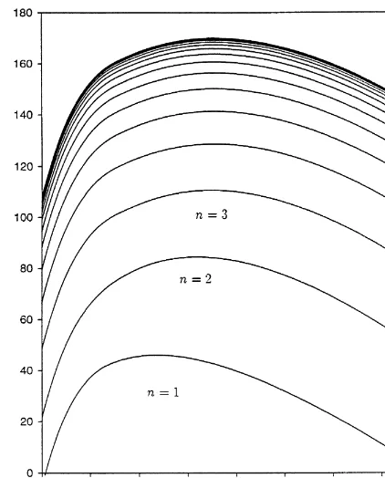
In order to demonstrate the transition from MM w
1 to MM
w
, we solved a 15-period problem under the same problem data, and compared the resultant expected pseudo-pro"t functions with the function we obtained by solving the in"nite horizon problem. Fig. 6 depictsMM w
n(0,qn) functions forn"1, 2,2, 15
andMM w
, which become indistinguishable from the pseudo-pro"t functions for largen, as predicted by the theory.
6. No-5xed-ordering-cost
In order to establish a link between this paper and the earlier studies reported in the literature, here we take a brief look at the model withK"0.
Following a similar inductive approach to the one we used previously, we suppose that MM w
1(0,q1) is
unimodal andPM w
n~1(in~1) is determined by a single-parameterpolicy:
PM w
n~1(in~1)"cin~1#
G
MM w
n~1(0,Sn~1), in~1)Sn~1,
MM w
Fig. 6. Expected pseudo-pro"t curves,MM w
n(0,qn) vs.qn, that are evaluated for the 15-period problem speci"ed in Section 6. The curve at the top represents the solution for the in"nite horizon model with the same parameter set. (It coincides with the expected pseudo-pro"t curves at largen.)
Under this setting, it follows from Eq. (6) that
MM w
n(0,qn)"max
G
G(0,pn,qn)#aMMw
n~1(0,Sn~1)
#a
qn~L(pn)
P
Sn~1
[MM w
n~1(0,x)!MM
w
n~1(0,Sn~1)]f(qn!x;pn) dx: pn3[Pl,P6]
H
. (15)It can be seen that for q
n)Sn~1, the integral drops out and we have
MM w
n(0,qn)"G
w (0,q
n)#aMM
w
n~1(0,Sn~1),
where Gw (0,q
n) is a unimodal function. ForSn~1(qn, however, we note that the integral in Eq. (15) is
negative-valued. Based on these observations, we establishMM w
n(0,qn) in two alternative ways, as shown in
Fig. 7. Considering Eq. (15) and Fig. 7, we discover that
minMS
g,Sn~1N)Sn)Sg, (16)
forn*2, and the con"guration shown in Fig. 7a can only occur forn"2. The recursive ordering in Eq. (16) implies that ifS
g)S1, thenSn"Sgfor alln*2. It is clear that ifv"c,
thenMM 1,G, andS
1"Sgby de"nition. But, it is more plausible, in general, thatv(c, in which caseS1will
be di!erent fromS
g.
Fig. 7. Construction ofMM w
n(0,qn) vs.qnforK"0; dashed curves representG w
(0,q
n) for: (a)Sg(Sn~1, and (b)Sn~1(Sg.
Intuitively, when the price is"xed,S
gmust be greater thanS1. Having the option of salvaging the leftovers
at a higher return, the decision maker will be encouraged to procure up to higher levels. But, under the impact of pricing, there could be a trade-o!between small-quantity high-price and large-quantity low-price scenarios. Demand uncertainty at a given level will then be contingent on the pricing decision. For this reason, under a general price-demand relationship, it is theoretically possible thatS
g(S1.
Fig. 7b shows that the expected pro"t level will be higher ifS
n~1shifts towardsSgand the contribution of
Gis more than the contribution of the negative valued integral in Eq. (15). Thus, overcoming the transient behaviour represented by Eq. (16), there will be a propensity, under the optimal solution, forS
nto approach
S
gSu$cient conditions for the optimality of a single-critical-number policy are given in [11]. In principle,as the number of periods is increased.
these conditions can be utilized to verify the form of the optimal procurement policy, but they are di$cult to interpret in terms of their managerial implications. Under some restrictions, Thowsen [11] shows that the single-parameter policy will be optimal if the demand is additive with a PF
2(Po&lyafrequency function of type
7. Non-stationary extensions
In addition to being dependent on price, it is possible that the demand distribution exhibits periodic shifts during the planning horizon due to seasonalities or changing market conditions. The natural way of incorporating such time-variability in our model would be to represent the demand in periodnby a random variable X
n(pn) with distribution Fn(x;pn). The generic function, now denoted by Gn, and the critical
parameters de"ned forGw
n, smgn(2(S6gn, would also be period-dependent.
By virtue of the fact that the demand distribution depends on price and the price can be set at the beginning of each period, extensions to time-dependent demand are immediate. It can be seen, going through the proofs in the appendix, that this does not alter the arguments and derivations, provided thatGw
n(0,qn) is
unimodal and the conditions6gn)skn~1
n~1holds for alln'1. This condition parallels the"xed-price version of
the non-stationary demand model [21,23] where it is assumed thatS
gn)Sgn~1forn'1. It can also be seen
that ifS
gn)s1n~1, thenkn"2.
Similarly, we can let the cost parameters and the discount factor depend on the period (i.e.,
c
n,rn,hn, Kn,an), without any di$culty, provided thatKn*an~1Kn~1(a0"1), andMM
w
1 is unimodal for
n'1 (which implies unimodality ofGw
n).
8. Deterministic demand
Under deterministic demand,X
n(p)"XM n(p) for alln. For technical reasons, we will assume thatXn(p) is
o(1/p) aspPRand aspP0`. Under this assumption, theriskless revenuefunctionR
n(p)"pXn(p) starts
growing at 0 whenp"0, reaches a maximum level, and declines down to 0 asptends to in"nity. We further assume that R
n(p) is a pseudoconcave function of pon (0,R) so that there is a unique breakeven point
between low-price-high-demand and high-price-low-demand situations in terms of revenue. It is shown in [19] that if X
n(p) is a convex or concave decreasing function, then Rn(p) is pseudoconcave on (0,R).
A detailed discussion of the properties of theriskles revenuefunction and related functions can be seen in [7,19].
UsingX
n(p)"XM n(p) in Eq. (3) we obtain
MM n(i
n, pn,qn)"Gn(in,pn, qn)#aMPM
w
n~1([qn!Xn(pn)]`)!c[qn!Xn(pn)]`N,
where
G
n(in,pn,qn)"(pn#r!c)qn!rXn(pn)!(pn#r#h!ac)[qn!Xn(pn)]`#cin. (17)
This representation leads to:
Corollary 4. ;nder deterministic demand, MM w
1(0,q1) is quasiconcave, and MM
w
n(0,qn) is quasi-K-concave for
n*2,where:
(i) MM w
n(0,qn) is increasing over qn3[0,Xn(Pnc)],n*2, where Pnc is the maximizer of (pn!c)Xn(pn) over
[Pl,P 6].
(ii) MM w
n(0,qn)*G
w
n~1(0,qn)#aMM
w
n~1(0,sn~1),MM
w
n(0,qn))G
w
n~1(0,qn)#aMM
w
n~1(0,sn~1)#aK, for qn'
X
n(Pnc)and n*2.
(iii) ¹he optimal inventory level is determined by the(s
n,Sn)policy:q
w
n"in#(Sn!in)d(sn!in).
This result was also obtained by Thomas [26], through a price-dependent lot-sizing approach. He demonstrated that there exists a positive integerm, wherem#1 is referred to as the planning horizon, such
that for all n, S
n"Xn(pHn)#Xn~1(pHn~1)#2#Xn~m(pHn~m), where pHn~j is the maximizer of
(p
n~j!en~j)Xn~j(pn~j), with
e
n~j"
C
c#hA
1# j~1+
k/1
(a
n~1an~22an~k)
BDN
(an~1an~22an~j),for 1)j)mandpH
n"Pnc.
Thus, sincee
n~(j`1)'en~j*cfor 1)j)m, it follows from Theorem A.1 in the appendix thatpHn"Pnc
and pHn~j"Pcn~j for 1)j)m; in particular, if X
n())"Xn~j()) for 1)j)m, then pHn"Pnc )pHn~1)pnH~2)2)pHn~m.
9. Conclusions
We established that a reorder-region, order-up-to-level procurement policy is optimal for the decision problem of interest in this paper, given thatMM w
1(0,q1) is unimodal, andin)s6gforn*2. Under this policy,
the vendor administers the best price in each period, whether or not an order is placed. We have also provided upper and lower bounds on the reorder and order-up-to levels, which should expedite the computational work, and su$cient conditions under which a reorder-point, order-up-to level policy is optimal.
Under the special case with deterministic demand, we have shown that the optimal ordering policy is determined by an (s,S) type policy, provided that the revenue functionR(p) is unimodal. For the in"nite horizon stationary model, we have provided a solution method that could be used to obtain the optimal solution numerically.
Furthermore, in the absence of a"xed ordering cost, the order-up-to levels are bounded from above byS
g,
and they are ordered in a non-decreasing fashion inn(see Eq. (16)). WithK'0, this ordering does not hold, however, andS
gis not necessarily an upper bound for order-up-to levels. For instance, we have obtained
S
1(Sg(S2(S5(S4(S3for the example problem withh"0.1 (see Tables 1 and 2).
One of the contributions of the paper is the solution method which is based on a non-derivative approach. Through this approach, we were able to develop distribution-independent and non-stationary results. The existing solution methods predominantly utilize the derivative approach, and impose restrictive assumptions on the demand distribution, the expected demand function, or the parameter set.
In terms of additional research that could follow the present e!ort, one interesting area is approximations. As a stationary approximation, we formulated the in"nite-horizon model in Section 5, and proposed an algorithm for it, based on the recursive solution of a sequence of renewal equations. It would be interesting to study the underlying convergence problems, both in terms of the proposed algorithm and the optimal control parameter values.
We have demonstrated that the optimal pricing trajectories,p
n(qn),n*1, can be complicated enough to
make the evaluation and administration of the optimal pricing strategy impractical. A simpler strategy, though not optimal, might be desirable in applications. One possibility is to approximate the best price by utilizing the single-period model characterized byG
n. That is,pg(qn)"argmaxMGHn(0,p,qn):p3[Pl,P6]N, for n'1. The functionMM n(0,p
g(qn),qn), as an approximation forMM
w
n(0,qn), would then be used recursively for
Appendix A
Proof of Theorem 1.Under the unimodality assumption aboutMM w
1(0,q1), it is su$cient to show, inductively,
that MM w
n(0,qn) satis"es conditions (a)}(f), given that MM
w
n~1(0,qn~1) does, since using the same line of
arguments in the proof, it can be trivially shown that MM w
2(0,q2) satis"es these conditions also. In what
follows, we haveq
n)sknn~1~1 unless speci"ed otherwise.
De"ning the`reorder regionaO
n~1for periodn!1 by
it follows under the inductive assumption aboutMM w
n~1thatPM
where the regionOMn~1is complementary to region O
n~1 with respect to [0,sknn~1~1]. Note thatOn~1is the
union ofk
n~1/2 reorder intervals.
We assume thatKis not exceedingly large so thats1
n~1'0. This assumption does not have any critical
in#uence on the results; it only decreases the number of terms to carry in the analysis and simpli"es the mathematical representation.
By considering Eq. (A.1), the integral in Eq. (3) can be rewritten as
qn~L(pn)
where the integral with respect to x3O
n~1W[0,qn!¸(pn)] represents the sum of integrals over the
compositexrangeO
n~1W[0,qn!¸(pn)]. Same is true forOM n~1W[0, qn!¸(pn)].
Using this result in Eq. (3) we obtain
which can be substituted in Eq. (5) to obtain
where it is understood thatq
n!¸(pn))snk~1n~1, which is also implied byqn)sknn~1~1.
This establishes (a). SinceGis a special case ofMM 1(withv"c), we considerGw
to be a unimodal function with a maximizer at S
g and a reorder level sg. Thus, under the inductive assumption that s1n~1(Sg, we
conclude from Eq. (A.3) that MM w
n(0,qn) is an increasing function of qn on [0,s1n~1]. Later, we shall
demonstrate that in facts1
n(Sgfor alln*2 (see the proof of Corollary 1).
a starting point. We rather start at Eq. (3). Since, under the inductive assumption, PM w
n~1(x))cx#MM
Therefore, it follows from Eq. (3) that
Under properties (b) and (c) we have
which indicates that MM w
n(0,qn) is bounded by two unimodal functions that are at most aK distance
(vertically) apart onq
n3[s1n~1,sknn~1~1].
Next, we consider the region [S
g,sknn~1~1]. Letq@n3(qn,R) be an arbitrary level for any givenqn3[Sg,sknn~1~1]. It
which implies that MM w
n(0,qn) is aK-decreasing over [Sg, sknn~1~1], and MM
On the other hand, it has been shown in [10] that lim
q1?=MM
Proof of Corollary 1.Evaluating Eq. (A.6) atq
Similarly, forq
Combining the above inequalities we get
Gw
Thus, considering the two boundary functions in Eq. (A.6) which can be represented by a pair of unimodal functionsaKdistance apart, and by indicating the critical inventory levelssmg(s
g(S
is an increasing function over [0,S
g], it follows from the proof of properties (a)}(c) in Theorem 1 that if
s
g(s11, thensg(s1n for alln'1.
Proof of Corollary 2.To initiate the inductive proof, we assume thatsl
It follows from the de"nition of G (see Section 4.1) that G(0,p
g] which is, in general, analytically
intractible. For this reason, we need to strengthen Eq. (A.9) in order to establish a veri"able su$cient condition.
SinceH(p
n,qn) is a continuous, convex increasing function inqnfor allpn, andLH(pn, qn)/Lqn"F(qn; pn), the
result in the Corollary is implied by Eq. (9) and Corollary 1.
Proof of Corollary 3.To initiate the inductive proof, we assume thats
1)Sg, which ensures thatMM
follows from Eqs. (3) and (5) that
MM w
Having this representation, we can proceed as follows:
which implies that
MM w
n(0,qn)*MM
w
n(0,q@n)!aK, (A.10)
if G(0,p
n(q@n), qn)!G(0,pn(q@n), q@n)*0. Note that Eq. (A.10) characterizes MM
w
n as aK-decreasing (which
implies that it isK-decreasing) over [S
g,R), and this leads to the desired result.
Derivation ofMM w
II(0,q). The solution of the renewal equation Eq. (14) is ([25]):
MM w
II(0,q)"G(0,pq, q)#a[1!F(q!s1;pq)]MM
w
(0,s1)#
q~L(pq)
P
s1
G(0,p
q,x)dRa(q!x;pq)
#aMM w (0,s1)
q~L(pq)
P
s1
[1!F(x!s1;p
q)]dRa(q!x;pq), (A.11)
whereR
ais determined by
R
a(x;p)"aF(x;p)#a
x
P
L(p)
F(x!u;p) dR
a(u; p).
We evaluateR
a(x; p) atx"q!s1andp"pq,
R
a(q!s1;pq)"aF(q!s1;pq)#a
q~L(pq)
P
s1
F(x!s1;p
q)dRa(q!x;pq),
which can be substituted in Eq. (A.11). Thus, we obtain
MM w
II(0,q)"G(0,pq, q)# q~L(pq)
P
s1
G(0,p
q, x) dRa(q!x;pq)
#aMM w
(0,s1)[1!F(q!s1;p
q)#Ra(q!s1; pq)#F(q!s1; pq)!Ra(q!s1;pq)/a]
"G(0,p
q, q)# q~L(pq)
P
s1
G(0,p
q, x) dRa(q!x;pq)#G
w
(0,s1)
C
a1!a!Ra(q!s1;pq)
D
.This implies the desired result.
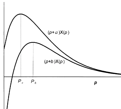
Proof of Corollary 4.Before we present the induction proof, we will establish the following property:
Property 1. ∀a,b with a'b, we have P
a)Pb where Pa"argsupM(p#a)X(p):p3(0,R)N and Pb"
argsupM(p#b)X(p):p3(0,R)N.
Fig. 8. Plots of the auxiliary functions (p#a)X(p) and (p#b)X(p) under an hypotheticalX(p) function.
IfP
a,Pb3(0,R), then they must satisfy the"rst-order conditionsA@(Pa)"0 and B@(Pb)"0. We rewrite
A(p) asA(p)"B(p)#(a!b)X(p), which leads toA@(p)"B@(p)#(a!b)X@(p). Evaluating the last equation at
p"P
awe get A@(Pa)"B@(Pa)#(a!b)X@(Pa), which implies
B@(P
a)"!(a!b)X@(Pa)'0. (A.12)
That is,B(p) is increasing atp"P
a. SinceB(p) is a pseudoconcave function we deduce thatPa)Pb. IfPaand
P
b are both non-interior point solutions, then Pa"Pb"0 since A(p)*B(p) for all p. If Pa"0 and
P
b3(0,R), then Pa)Pb. Finally, if Pa3(0,R), then from Eq. (A.12) we conclude that Pa)Pb. Hence,
P
a)PWe identifybin any case.P
ncas the maximizer of (p
n!c)Xn(pn) over [Pl,P6]. That is,Pnc"minMmaxMPMnc,PlN, P6Nwhere PMnc is the maximizer of (p
n!c)Xn(pn) over (0,R). Similarly, Pnh, Pnhc and Prc are the maximizers of
(p
n#h!v)Xn(pn), (pn#h!ac)Xn(pn) and (pn!r!ac)Xn(pn) over [Pl,P6], respectively. Since!c)h!v, !c)h!acand!r!ac)!c, it follows from Property 1 thatPnc*Pnh,Pnc*PnhcandP
rc*Pnc. That is,
X
nNow we can establish the proof of Corollary 4. It is shown in [19] that(Pnc))Xn(Pnh), Xn(Pnc))Xn(Pnhc) andXn(Pnrc))Xn(Pnc). GH
n(0,qn) is quasiconcave with
S
n"Xn(Pnc). Having this in mind, assume thatMM
w
n~1(0,qn~1) satis"es (i) and (ii) in Theorem 2. Thus, there
exists single reorder and order-up-to levels for periodn!1. That is,k
n~1"2. Using this result, we obtain
MM n(i
n, pn,qn)"Gn(in,pn,qn)#a
G
MM w
n~1(0,sn~1), [qn!Xn(pn)]`(sn~1,
MM w
n~1(0, [qn!Xn(pn)]`), sn~1)[qn!Xn(pn)]`.
(A.13)
First, we represent then-period pseudo-pro"t function asMM w
n(0,qn)"maxMMM (1)n (0,qn),MM (2)n (0,qn)N, where
MM (1)
n (0,qn)"maxMMM n(0,pn, qn):Pl)pn)pNnN,
MM (2)
n (0,qn)"maxMMM n(0,pn, qn):pNn)pn)P6N,
and pNn is de"ned by X
n(pNn)"maxMminMqn, Xn(Pl)N,Xn(P6)N. That is, pNn"Pl if qn*Xn(Pl), pNn"P6 if q
n)Xn(P6); otherwise,pNnis the unique solution ofXn(pNn)"qn. Note that ifpn3[Pl, pNn), thenqn)Xn(pn) and
if p
n3(pNn,P6], then qn*Xn(pn). Therefore, MM (1)n and MM (2)n represent the n-period pseudo-pro"t values
under the best pricing policy that results in no leftovers and no shortages, respectively, at the end of period
nfor a givenq
n. In what follows, we work with these complementary subproblems to analyseMM
w
n(0,qn) on
variousq
nranges and then combine our"ndings to complete the proof.
It follows from Eqs. (A.13) and (17) that,MM (1)
n (0,qn)"aMM
w
n~1(0,sn~1)!cqn#maxMpnqn!r(Xn(pn)!qn):
Pl)p
n)pNnN, where the maximand is an increasing function ofpn. Hence, we obtain
MM w
We shall demonstrate that MM (21)
n and MM (22)n are both increasing on [Xn(P6),Xn(Pnc)] which implies that
MM (2)
n is also increasing over the sameqnrange.
Next, we shall analyseMM (22)
n . Note that forqn)Xn(P6)#sn~1, we havepLn"P6andMM (2)n "MM (21)n . Thus,
we need to consider MM (22)
n (0,qn) only on [Xn(P6)#sn~1,R).
We identify q@
n arbitrarily with Xn(P6)#sn~1)qn(qn@)Xn(Pnc) to show that MM (22)n (0,qn)(
MM (22)
n (0,q@n). Let p be the maximizer in Eq. (A.16) which satis"es pLn)p)P6. Then, de"ne pL@n by
q@
n!sn~1"Xn(pL@n), andp@byqn!Xn(p)"q@n!Xn(p@). Thus, we have
q@
n!Xn(p@)"qn!Xn(p)*sn~1"q@n!Xn(pL@n),
which impliesPnc)pL@
n)p@(p)P6. Considering the order of these critical prices and observing Fig. 8 we
write
MM (22)n (0,q
n)"aMM
w
n~1(0,qn!Xn(p))!(c#h!ac)qn#(p#h!ac)Xn(p)
"aMM w
n~1(0,qn!Xn(p))!(c#h!ac)[qn!Xn(p)]#(p!c)Xn(p)
"aMM w
n~1(0,q@n!Xn(p@))!(c#h!ac)[q@n!Xn(p@)]#(p!c)Xn(p)
(aMM w
n~1(0,q@n!Xn(p@))!(c#h!ac)[q@n!Xn(p@)]#(p@!c)Xn(p@)
)maxMaMM w
n~1(0,q@n!Xn(pn))!(c#h!ac)q@n#(pn#h!ac)Xn(pn): pL@n)pn)P6N "MM (22)
n (0,q@n),
which indicates thatMM (22)
n is an increasing function ofqnover [Xn(P6)#sn~1, Xn(Pnc)].
We have so far shown thatMM (21)
n andMM (22)n are increasing inqnover [Xn(P6),Xn(Pnc)]; thus,MM (2)n ("MM
w
n) is
also increasing inq
nover the same range.
The next q
n region will be [Xn(Pnc),Xn(Pnhc)#sn~1]. We have MM
w
n~1(0,qn!Xn(pn)))
MM w
n~1(0,Sn~1) for all feasiblepnandqnvalues. In addition, sincePnhc)pLn, (pn#h!ac)Xn(pn) is decreasing
over [pLn,P
6]. Hence, we have MM (22)
n (0,qn))maxMaMM
w
n~1(0,Sn~1)!(c#h!ac)qn#(pn#h!ac)Xn(pn):pLn)pn)P6N )maxMaMM w
n~1(0,Sn~1)!(c#h!ac)qn#(pn#h!ac)Xn(pn):pNn)pn)pLnN
"MM (21)n (0,q
n)#aKn~1,
which implies thatMM (2)n (0,q
n), given by Eq. (A.6), is bounded byMM (21)n (0,qn) andMM (21)n (0,qn)#aKn~1, where
MM (21)
n is decreasing (see Eq. (A.17)). Hence, MM (2)n (0,qn) is an aKn~1-decreasing function over
[X
n(Pnc),Xn(Pnhc)#sn~1].
Consider nowX
n(Pnhc)#sn~1)qn. In this range,pL@n)pLn)Pnhc. Hence, (pn#h!ac)Xn(pn) is increasing
over [pL@
n,pLn]. In addition, under the inductive assumption,MM
w
n~1(0,qn!Xn(pn)) isKn~1-decreasing inqnfor
X
n(Pnhc)#sn~1)qnwithpLn)pn. Hence, we have
MM (22)
n (0,qn)"maxMaMM
w
n~1(0,qn!Xn(pn))!(c#h!ac)qn#(pn#h!ac)Xn(pn): pLn)pn)P6N "maxMaMM w
n~1(0,qn!Xn(pn))!(c#h!ac)qn#(pn#h!ac)Xn(pn): pL@n)pn)P6N *maxMa[MM w
n~1(0,q@n!Xn(pn))!Kn~1]!(c#h!ac)qn#(pn#h!ac)Xn(pn):pL@n)pn)P6N 'maxMaMM w
n~1(0,q@n!Xn(pn))!(c#h!ac)q@n#(pn#h!ac)Xn(pn):pL@n)pn)P6N!aKn~1
"MM (22)
n (0,q@n)!aKn~1,
which implies that MM (22)
n is aKn~1-decreasing. Since MM (21)n (0,qn) is decreasing over [Xn(Pnhc)#sn~1,
X
n(Pl)#sn~1] (see Eq. (A.17)),MM (2)n (0,qn) isaKn~1-decreasing over [Xn(Pnhc)#sn~1,R).
Finally, to complete the continuity we need to consider q
n"Xn(Pnhc)#sn~1. Since MM
w
n~1(0,Sn~1) and
(Pnhc#h!ac)X
n(Pnhc) are the global maximas of their respective functions, and MM (21)n is decreasing over
[X
n(Pnc),Xn(Pnhc)#sn~1], we obtain from Eq. (A.17) that
MM (2)
n (0,qn)*MM n(21)(0,qn)"a(MM
w
n~1(0,Sn~1)!Kn~1)!(c#h!ac)qn#(Pnhc#h!ac)Xn(Pnhc)
*MM (2)
n (0,q@n)!aKn~1,
for allq@
n'qn"Xn(Phc)#sn~1.
Therefore, the proof follows by combining the results for the entireq
nrange.
References
[1] K.J. Arrow, T. Harris, J. Marschak, Optimal inventory policy, Econometrica 19 (1951) 250}272. [2] T.M. Whitin, Inventory control and price theory, Management Science 2 (1955) 61}68. [3] E.S. Mills, Uncertainty and price theory, Quarterly Journal of Economics 73 (1959) 116}130. [4] E.S. Mills, Price, Output, and Inventory Policy, Wiley, New York, 1962.
[5] S. Karlin, R.C. Carr, Prices and optimal inventory policy, in: K.J. Arrow, S. Karlin, H. Scarf (Eds.), Studies in Applied Probability and Management Science, Stanford University Press, Stanford, CA, 1962.
[6] A.J. Nevins, Some e!ects of uncertainty: Simulation of a model of price, The Quarterly Journal of Economics 80 (1966) 73}87. [7] A.L. Hempenius, Monopoly with random demand, Rotterdam University Press, Rotterdam, 1970.
[8] E. Zabel, Monopoly and uncertainty, Review of Economic Studies 37 (1970) 205}219.
[9] E. Zabel, Multiperiod monopoly under uncertainty, Journal of Economic Studies 5 (1972) 524}536.
[10] E. Zabel, Price, output and inventory behavior with a general demand structure, in: The Economics of Inventory Management, Elsevier, Amsterdam, 1988, pp. 319}332.
[11] G.T. Thowsen, A dynamic nonstationary inventory problem for a price/quantity setting"rm, Naval Research Logistics Quarterly 22 (1975) 461}476.
[12] L. Young, Price, inventory and the structure of uncertain demand, New Zealand Journal of Operational Research 6 (1978) 157}177.
[13] L. Young, Uncertainty, market structure, and resource allocation, Oxford Economic Papers 46 (1979) 47}59. [14] L.J. Thomas, Price and production decisions with random demand, Operations Research 22 (1974) 513}518.
[15] G. Gallego, G. Van Ryzin, Optimal dynamic pricing of inventories with stochastic demand over"nite horizons, Management Science 40 (1994) 999}1020.
[16] N.C. Petruzzi, Learning models for pricing and inventory control under uncertainty, Ph.D. Dissertation, Department of Management, Purdue University, West Lafayette, IN, 1995.
[17] S. Subrahmanyan, R. Shoemaker, Developing optimal pricing and inventory policies for retailers who face uncertain demand, Journal of Retailing 72 (1996) 7}30.
[18] E.L. Porteus, Stochastic inventory theory, in: D.P. Heyman, M.J. Sobel (Eds.), Handbooks in OR and MS, vol. 2, Elsevier, North-Holland, 1990.
[19] H. Polatoglu, Optimal order quantity and pricing decisions in single-period inventory systems, International Journal of Production Economics 23 (1991) 175}185.
[20] H. Scarf, The optimality of (s,S) policies in the dynamic inventory problem, in: Mathematical Methods in the Social Sciences, Stanford University Press, Stanford, CA, 1960.
[21] A.F. Veinott, On the optimality of (s,S) inventory policies: new conditions and a new proof, SIAM Journal of Applied Mathematics 14 (1966) 1067}1083.
[22] E.L. Porteus, On the optimality of generalized (s,S) policies, Management Science 17 (1971) 411}426.
[23] M. SchaKl, On the optimality of (s,S)-policies in dynamic inventory models with"nite horizon, SIAM Journal of Applied Mathematics 30 (1976) 528}537.
[24] A. Lau, Hing-Ling, Lau Hon-Shiang, The newsboy problem with price-dependent demand distribution, IIE Transactions 20 (1988) 168}175.
[25] I. Sahin, A generalization of renewal processes, Operations Research Letters 13 (1993) 259}263.