in the Great Depression
Ali Anari and James Kolari*
The credit hypothesis maintains that nonmonetary factors worsen declines in output during severe economic contractions, which has been a prominent rationale for stringent bank regulation. We apply recent advances in time series analysis to re-examine the role of U.S. bank failures in the Great Depression. In brief, month-by-month decompositions of output, prices, money supply, the liabilities of failed firms, and the deposits of failed banks indicate that bank failures did not initiate the fall in output and prices. However,
chronicbank failure over at least a two-year period, in combination with a surge in failures in the latter part of this period of banking industry distress, had large negative effects on all of the variables under study. We conclude that chronic bank failures coupled with subsequent threshold failure effects can have deep and pervasive influences on the economy, which justify government intervention at such times. © 1999 Elsevier Sci-ence Inc.
Keywords:Bank failure; Economic output; Great Depression
JEL classification:E44, G21, N22
I. Introduction
Bernanke (1983) first proposed the credit hypothesis to help explain the collapse in U.S. economic productivity during the Great Depression. In brief, this hypothesis argues that bank failures have nonmonetary effects on the economy which disrupt credit flows in the financial intermediation process and, thereby, exacerbate declines in economic activity. An extreme case is the possibility of a banking crisis in which serious damage to the financial system is possible, i.e., loss of public confidence and resultant runs on insolvent banks that spread to solvent banks, which is known as the contagion effect [see Kaufman
*Center for Business and Economic Research, Texas A & M University, College Station, Texas; Finance Department, Texas A & M University, College Station, Texas
Address correspondence to: Dr. James W. Kolari, Finance Dept., Texas A&M University, College Station, TX 77843.
(1994)]. To protect themselves, solvent banks not only shift funds to liquid assets but curtail lending, due to rising firm bankruptcies, which causes a lemons problem in the credit market [see Diamond and Dybvig (1983)]. In this sense, bank failures are perceived as more damaging to the economy than the failure of other firms, and in the words of Kaufman (1996, p. 25), “ . . . almost all countries have imposed special prudential regu-lations on banks to prevent or mitigate such adverse effects.”
Indeed, the Great Depression promulgated a panoply of U.S. banking regulations under the 1933 and 1935 Banking Acts which covered a broad array of issues, including pricing, products, and geographic expansion. Whereas the Great Depression witnessed the failure of some 9,000 banks between 1929 and 1933, and the loss of about 25% of bank system deposits [see Bernanke (1983) and Wheelock (1995)], the post-Depression regulatory blanket preserved a more or less steady state of about 15,000 banks until 1980. At that time, increasing interest rate volatility, financial innovation, and new competition from nonfinancial firms began to motivate deregulation of Depression-era banking laws. Today, bank deposit and loan interest rates are totally deregulated, many restrictions on securities and insurance products are relaxed, and interstate banking is permitted. In turn, the number of bank failures per year has noticeably increased at times. For example, in the years 1987 to 1989, the number of failed banks plus failing banks involved in regulator-assisted mergers exceeded 200 per year [see Boyd and Graham (1996)]. Recent work by Mason (1998) compared the direct and indirect costs of large (or national) bank failures in the Great Depression with the bank failure episode in the late 1980s and early 1990s in the United States. He calculated that FDIC disbursements to closed banks jumped in recent years, e.g., between 1988 and 1992, disbursements exceeded $10 billion per year and peaked in 1991 at about $20 billion. Mason (1998) found similarities in these two periods of banking distress, in terms of substantially lower recovery rates from closed banks, and concluded that potential macroeconomic losses due to asset market overhang and/or inefficient management of failed bank assets can be significant. An important empirical issue in this respect is the sensitivity of real economic activity to bank failures. Do bank failures have immediate short-run negative effects on output, or are they associated with long-run effects? How important are the effects of bank failures on output relative to other factors, such as prices and money supply? Answers to these questions are relevant to the continued deregulation of the banking industry to the extent that there is compelling empirical evidence with respect to the credit hypothesis.
With this motivation in mind, the present paper seeks to contribute further empirical evidence on the credit hypothesis by revisiting the Bernanke (1983) study. He and others [e.g., see Calomiris et al. (1986); Gertler (1988); Haubrich (1990)] employed a single-equation time series regression approach to examine short-run interactions between key economic and financial variables. Unlike those studies, we have applied the more sophisticated econometric methods of vector autoregression (VAR) and cointegration analysis [see Johansen (1988, 1991)]. These methods are superior to single-equation time series models because they fully incorporate the dynamic relationships among all the variables under investigation. Rather than basing our inferences on a few coefficients in a single regression equation (viz., about 12 coefficients) that reflects the relationships of the variables throughout the entire period of observation, we employed five equations which each contain five variables with 12 monthly lags. The historical decompositions of
time series variables provide valuable information about the time path of the impact of each variable on the rest of the variables under investigation. Information about the month-by-month impact of each variable, with respect to the other variables in the model, are particularly useful in sorting out their relative contribution in explaining the declines in output, prices, and money supply.
Based on data used in the Bernanke (1983) study, and historical decompositions of the time series variables in the VAR model, our results indicate that bank failures did not play an important role in explaining the drop in output until the last few months of the Great Depression episode. In this regard, persistent bank failures over at least a two-year period which escalated over time did contribute to output declines. Importantly, the VAR model results reveal thatchronicand increasing bank failures had severe negative impacts on not only output but prices, money supply, and business failures. The policy implication of these findings to banking regulation is that bank failures by themselves do not necessarily have deleterious effects on the economy; however, chronic and severe bank failures seriously disrupt the financial intermediation process and potentially have pervasive adverse effects on the economy. Corroborating evidence for this inference is the finding by Mason (1998) that failed bank assets are liquidated more slowly and with lower recovery rates during periods of financial crisis. Consequently, at some point, government intervention is justified to stabilize the banking system. Although a direct link to current banking issues is not possible, these findings tend to suggest that, as long as there is a lender of last resort (i.e., the central bank) to overcome the problem of chronic and deepening failures, isolated failures of individual institutions in the context of today’s more competitive banking environment do not appear to be a major problem with respect to economic productivity.
The next section overviews related empirical literature. Section III describes the Johansen (1988, 1991) cointegration procedure and the data. Section IV reports the empirical results, and the last section contains conclusions and implications.
II. Related Literature
Friedman and Schwartz (1963) argued that banking panics in the Great Depression reduced the money supply, which they found to be highly correlated with the dramatic decline in U.S. output. In contrast to this monetarist view of the causes of the Great Depression, Gurley and Shaw (1955) argued that bank failures were an important explanatory factor for reasons of credit intermediation services, i.e., the so-calledcredit hypothesis. Empirical work by Bernanke (1983) tended to support the notion that, apart from their role in the money supply process, bank failures raised the cost of credit intermediation and thereby lowered business investment and output.
The landmark study of Bernanke (1983) empirically tested the credit hypothesis by using a Lucas-Barro type model to initially examine the effects of money shocks and price shocks on real output in two separate regressions. Price surprises were found to have a stronger relationship to output than money surprises. More importantly, although both
effects were statistically significant, they explained only about half of the decline in output during the period 1930 –1933.
Based on this evidence, Bernanke (1983) argued that there was an error of omission in the monetary model and, subsequently, sought proxies for nonmonetary factors affecting output. Two key proxies were selected: the liabilities of failed businesses and the deposits of failed banks. In both the money shocks and price shocks regression models, these nonmonetary variables and lagged first differences were significant, and the money and price coefficients were unchanged for the most part. Bernanke (1983, p. 270) concluded that “ . . . nonmonetary effects of the financial crisis augmented monetary effects in the short-run determination of output.” In general, inclusion of the nonmonetary proxies for the financial sector predicted a more severe and longer decline in output than would be predicted by models of monetary contraction alone. Bernanke (1983) further observed that the Great Depression was a global crisis and that countries experiencing bank crises (i.e., the United States, Germany, Austria, Hungary, and others) suffered the most severe economic downturns.
Studies by Calomiris et al. (1986) and Gilbert and Kochin (1989) tested the effects of U.S. bank failures on regional economic activity. Calomiris et al. examined farm output data from the period 1977–1984 for different states, while Gilbert and Kochin focused on economic activity as measured by both the state sales tax and employment during the period 1981–1986 in Kansas and Nebraska. Both studies found that bank failures signif-icantly affected economic activity, thereby contributing evidence in support of the credit hypothesis.
More recent literature has been directed to international comparisons of banking crises and macroeconomic effects. For example, Bernanke and James (1991) examined data from a panel of 24 countries and found that the length of banking panics significantly affected industrial production. Importantly, the authors argued that differences between countries’ banking crises were related to institutional and policy differences, which implies that banking panics were not entirely explained by macroeconomic downturns alone but, instead, had an independent macroeconomic effect. The significance of the length of banking panics was further supported by a related paper by Bernanke and Carey (1994), who collected data for 22 countries. Bernanke (1995) has overviewed these studies in more detail.
Another branch of literature examines the general role of bank credit, as opposed to bank failures and associated credit disruptions, on economic activity. For example, King (1985) used vector autoregression (VAR) techniques to test the credit hypothesis in non-Depression years and found mixed results based on aggregate U.S. data. Also, Samolyk (1990) tested data on past insolvencies of corporate and noncorporate borrowers in Great Britain and found evidence in support of the credit view. This more general approach to testing the credit hypothesis was supported by theoretical work by Bernanke and Gertler (1987). They argued that there is a link between economic growth and the health of the financial system. In the macroeconomic model developed by the authors, investment and output were determined by the “willingness of banks to undertake risky projects,” which in turn is determined by the net capital of the banking system. Of course, net bank capital would be impaired by unexpected loan losses and, subsequently, reduced credit availability could further slow economic activity.
Another theoretical proposition by Bernanke and Gertler (1987b) is that information asymmetries between lenders and entrepreneurs can, at times, cause higher costs of capital to firms and cause decreased investment and economic output. At times of financial distress, there is increased demand for loans from low-quality borrowers, which creates a lemons problem for lenders attempting to sort out low- and high-quality firms. A lemons premium is subsequently added to the cost of capital, which diminishes efficient invest-ment and, in severe circumstances, can lead to an investinvest-ment collapse. For those inter-ested, Gertler (1988) provides an in-depth survey of the interaction between the financial sector and real economic output, with particular emphasis on the production and transfer of information in the credit process. Another more recent survey of theory and empirical research by Levine (1997), which draws a close linkage between the functioning of the financial system and long-run economic growth, cites international comparisons as supporting evidence.
The importance of the credit hypothesis rests in its policy implications. As Moore (1997) has observed, the policy debate centers on the extent to which government should respond to financial crises. On the one hand, government intervention can create a moral hazard problem, in which banks increase risk-taking due to their limited liability for losses. The result of excessive government assistance is greater systemic risk in the banking industry than otherwise. By contrast, it can be argued that there are no close substitutes for bank credit, as banks provide unique information production services to the financial market. Government assistance is recommended in this instance to sustain the supply of credit to firms and prevent an economic collapse due to a credit crunch. Apparently, this latter viewpoint motivated U.S. policy after the Great Depression. The Banking Acts of 1933 and 1935 introduced heavy regulation of banks to reduce compe-tition and preserve the safety and soundness of the banking industry.
More recently, as cited by Moore (1997), U.S. policy has shifted away from govern-ment assistance as a way to control bank risk. Today, under the Federal Deposit Insurance Corporation Improvement Act of 1991 (FDICIA), government regulation is linked to bank capital, and prompt corrective action guidelines reduce regulators’ ability to forbear bank condition problems. Thus, while the credit hypothesis had its roots in the Great Depres-sion, it has contemporary significance from a policy perspective. In this respect, an anonymous referee noted that, if bank failures have immediate effects, then rapid policy responses in the context of a fairly strict regulatory environment are needed. Alternatively, if occasional bank failures do not have short-run effects, then policy makers need not intervene unless chronic or a large surge in failures threatens the credit intermediation process. In the latter case, weak banks can be allowed to fail, sometimes in large numbers (as in the 1980s and early 1990s) without important macro consequences or the need for undue regulatory burdens.
In the forthcoming section, we overview an empirical methodology that has the advantage of providing some insights into short-run versus long-run effects between bank failures and economic output during the U.S. Great Depression.
III. Methodology
In the present paper, we use the same variables and sample period during the U.S. Great Depression as Bernanke. The variables are, namely, an index of industrial production (IN), wholesale price index (PX), nominal money stock (MS), liabilities of failed businesses (LB), and the deposits of failed banks (DB). The index of industrial production and money supply (M1) are seasonally adjusted, and the liabilities of failed businesses and deposits of failed banks are deflated by the wholesale price index. A logarithmic transformation of all variables is used. The sample data is monthly and covers the period January 1921 to December 1941. It should be noted that the deposits of failed banks do not measure lost deposits to the extent that deposits of failed banks are shifted to other banks. Recent evidence by Mason (1998) indicates that payouts to depositors of failed banks during the Great Depression were only about 30%– 40% in the year of failure. In subsequent years, recoveries due to restorations to solvency and assisted mergers (i.e., purchase and assumption resolutions) yielded eventual payouts of about 80% of deposits over five or more years. Interestingly, Mason (1998) found that these statistics are similar in level and time pattern to the bank failure episode of the late 1980s and early 1990s. Comparing the two periods, he observed that the disposition of bank assets in the resolution process can cause significant macro-economic losses. We infer that bank failures seriously disrupted the credit intermediation process for an extended period of time during the Great Depression. For our purposes, as observed by an anonymous referee, it should be recognized that the deposits of failed banks is a proxy for unobservable lost deposits, which are assumed to be a constant percentage over time. Also, consistent with the arguments of Bernanke (1983), this variable is a proxy for the degree of disruption in the bank credit intermediation process. Unlike the single equation method used in Bernanke (1983), the VAR methodology employed here generates the historical decomposition of the variables under investigation, which shows the monthly estimates of each variable’s influence on all other variables. Thus, VAR provides additional detail on the economic and financial interactions during the Great Depression.
The reduced form associated with equation (1) is given by:
Yt5
O
represents the unexpected movements in variables in vectorY. In reduced form, VAR has no contemporaneous term, such that each equation is estimated by ordinary least squares (OLS) method.
decom-positions are estimated based on the following partition of the moving average represen-tation of the variables in the system:
YT1J5
O
s50 j21AsuT1j2s1@XT1jb1
O
s5j`
AsuT1j2s#, (3)
where¥sj2510
AsuT1j2srepresents that part ofYT1Jdue to innovations in periodT1 1 to T1j, and the term [z] is the forecast ofYT1Jbased on information available at timeT. XT1jis the deterministic part of the model (e.g., a constant or time trend term). We should
comment that the forecasts are in-sample (as opposed to out-of-sample) and, therefore, are intended to provide insights into how shocks in one variable (e.g., a sharp decline in the deposits of failed banks) affected other variables (e.g., economic output).
Prior to estimating the vector autoregressions, we employed unit root tests to determine whether the data were stationary, as well as the Johansen trace test for cointegration. Cointegration tests help to determine whether the VAR model must be estimated in level or first difference, or structured in the class of vector error-correction (VEC) models. The Johansen (1991) procedure starts with thekth order unrestricted VAR model in equation (2) and transforms it to the VEC representation:
DYt5m 1
O
i k21GiDYt2i1
P
Yt2k1et, (4)where
Gi52I1pt1p21. . .1pi;
P
52I1pt1p21. . .1pk forI51, . . . , k21;m 5n31 vector of intercepts;
et5PNp~0, s!.
The difference between the VAR model in equation (2) and the VEC model in equation (4) is the term P. The coefficient matrix, P, conveys information about long-term relationships among the variables and lends itself to hypothesis testing. There are three possible cases: 1) if matrixPis of full rank,Yis a stationary system (i.e., all elements of
Yare stationary in levels); 2) if the matrixPhas rank zero, all variables inY have unit roots and equation (4) is simply a difference vector time series model; and 3) in the intermediate case, when 0,rank(P)5r,n, there arercointegrating relations among the variables. In case (3), rankr, nimplies that P 5ab9, wherea andbare n3 r
matrices, andris the number of cointegrating relationships [see Johansen (1991)]. Theb matrix is made up ofrcointegration vectors that satisfy equation (4), and the amatrix contains error correction parameters.
IV. Empirical Results
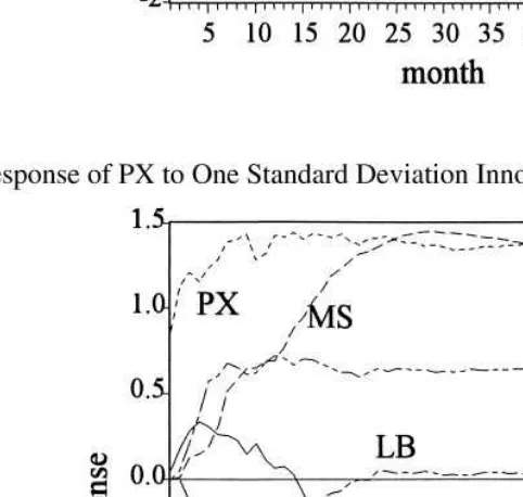
The modeling procedure started with the tests of integration and cointegration. The procedure requires that the time series variables under investigation be integrated of order zero or one. Augmented Dickey-Fuller (ADF) and Phillips-Perron tests described in the Appendix were used to determine the order of the integration of the variables. Table 1 reports the results of the unit root tests on the levels as well as the first differences of the variables. These tests suggest thatIN,PX,MS, andLBare integrated of order one, which means that these variables are nonstationary in levels but stationary after first differences. By contrast,DBis integrated of order zero and is stationary in level. Thus, these variables satisfy the necessary conditions for use in the Johansen system.
For the cointegration test, we used the Johansen (1992) sequential test procedure to determine the number of cointegrating vectors and whether a constant term should be included in the error-correction representation within or outside matrix P. Because this test is sensitive to the number of lags, researchers ordinarily set the number of lags equal to the periodicity of the data (e.g., four lags for quarterly data) or base the lag length on a criterion such as the Akaike Information Criteria [see Akaike (1973)] and the Schwarz Criterion [see Schwarz (1978) and Hafer and Sheehan (1991)]. As our data are monthly observations, we included 12 monthly lags in the Johansen tests and in the estimated VAR models. Using this lag length, the test results in Table 2 suggest the existence of two cointegrating vectors.
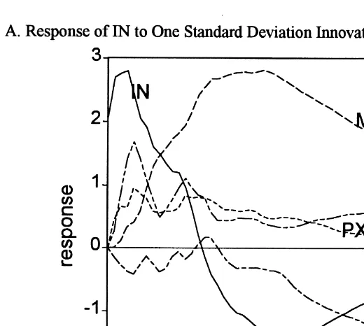
Two models were then estimated with the same lag length: a vector error correction model with two cointegrating vectors and a VAR model in levels of the variables. The complete estimates of these models are available upon request from the authors. Using Choleski decomposition of the covariance matrix, the impulse response functions gener-ated from the two models were estimgener-ated to examine whether the models were identified. The results from the impulse responses generated from the VAR and VEC models are illustrated in Figures 1 and 2, respectively. As shown there, the direction of the responses of industrial output and prices to one standard deviation shock in these variables indicates
5A problem with the bank deposit series is that the deposits of banks suspended in March 1933 were seven times that of the next worse month. Bernanke (1983) made an adjustment by scaling down the figure to 15% of the actual deposits of failed banks in March 1933. We found the univariate properties of the deposits of failed banks sensitive to the magnitude of the March 1933 observation; for instance, if we take 15% of the actual observation, then the series is integrated of order one. We also ran the model with the scaled-down figure, but the model was not identified when the impulse response functions were examined. Subsequently, we used the actual figure for March 1933 deposits of failed banks.
Table 1. Unit Root Test Results
Variablea ADF Za Zt Variablea ADF Za Zt
IN 20.58 1.10 1.44 DIN 28.19 2118.61 29.94
PX 21.58 20.22 20.57 DPX 27.94 2166.12 211.11
MS 0.25 1.15 3.18 DMS 28.11 2391.06 216.50
LB 21.40 23.30 21.52 DLB 215.88 2275.50 229.43
DB 23.74 2250.97 214.93 DDB 218.97 2294.97 266.50 aVariable definitions:
that the signs of price and quantity are consistent with the supply and demand equations. Notice that the differences between the results for the VEC and VAR models are small in magnitude up to 24 months in the forecast horizon and thereafter increase for longer horizons. Also, Table 3 indicates that Akaike and Schwarz criteria support the selection of the VAR (as opposed to the VEC) model. Because the cointegrating restrictions are asymptotically satisfied by levels VAR, and the two models’ results are similar (especially for short term horizons), the VAR model was selected for the estimation of the historical decomposition of the variables during the Great Depression.
An anonymous referee suggested that we check the robustness of the results to alternative variable ordering schemes. These additional analyses yielded the same results for the most part, and are available from the authors upon request. In our opinion, economic reasoning best supports our recursive ordering of industrial production, price, money supply, liabilities of failed businesses, and deposits of failed banks. If we had placed the latter nonmonetary variables first in order, the index of industrial production would have been more greatly influenced by them than the present ordering. Hence, our ordering scheme provides conservative estimates of the influence of the nonmonetary variables on economic output.
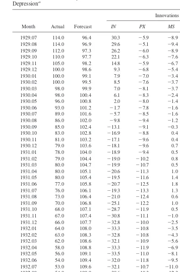
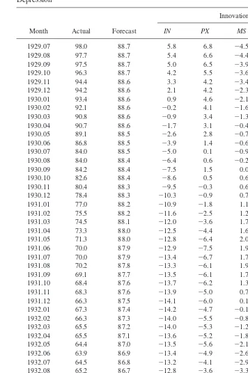
Tables 4 – 8 report the month-by-month decompositions of the variables beginning with the slide in output, prices, and money supply in July 1929 until August 1933. The bank holiday in March 1993 marks the beginning of massive government intervention, such that it is difficult to infer the effects of bank and business failures on output after this month. The actual level of each variable is shown in the first column, and the second column gives the forecasted level generated by the VAR model. As shown in the remaining columns, the differences between actual and forecasted levels were explained by innovations (or shocks) in each of the variables in the model. For example, referring to the first line in Table 4, when the decline in output began in July 1929, the actual output was higher than the expected output by 17.6 units, due to a 30.3 unit positive own shock in output, as well as 5.9 and 8.0 unit negative shocks in prices and money supply, respectively. The unit shocks in liabilities of failed businesses and deposits of failed banks are 0.0 and 2.0, respectively, which reflects a negligible nonmonetary effect in the beginning of the Depression. From July 1929 to March 1930, the negative shocks in prices and, in particular, in money supply were responsible for slowing down the growth of output. By
6We only report results for the focal Great Depression episode 1929–1933 rather than the entire sample period 1921–1941 to conserve space. President Roosevelt announced a national bank holiday in March 1933, after which the number of bank failures substantially declined (e.g., over 95% of the deposits of failed banks in 1933 occurred in the first quarter of that year, and no more than 60 banks failed in any year after this unprecedented event). Results for the entire period are available upon request from the authors.
Table 2. Johansen’s Maximum Eigenvalue and Trace Tests
Eigenvalue
Eigenvalue Test Trace Test
Test Statistics 90% Critical Value Test Statistics 90% Critical Value
0.223 60.49 20.90 97.87 64.74
0.078 19.54 17.15 37.38 43.84
0.050 12.31 13.39 17.85 26.70
0.022 5.52 10.60 5.54 13.31
June 1930, output started to suffer from its own negative shocks, as well as negative price shocks, whereas money supply shocks diminished considerably. From June 1930 to November 1931, the slide in output is mainly explained by negative own shocks as well as negative price shocks. From November 1931 to August 1933, negative shocks in money supply surpassed price shocks in explaining output declines as well as own shocks by the end of the period.
Relevant to the credit hypothesis, the liabilities of failed businesses had little or no negative impact on output declines in the period under study. By contrast, the deposits of failed banks did not negatively affect output from July 1929 to January 1932, but thereafter began to gradually increase in importance in explaining the decline in output. In the period February 1932 to March 1933, negative shocks to the deposits of failed banks gradually increased in terms of their effect on output declines. Focusing on March 1933, actual output stood at 54.0 units, or 57.3 units below the expected output, which is explained by 19.2, 10.7, 17.5, and 11.9 unit negative innovations in output, prices, money supply, and the deposit of failed banks, respectively (as well as a 2.0 positive unit innovation in the liabilities of failed businesses). Notice that the influence of deposits of failed banks exceeded prices at that time. We infer from these results that bank failures did not initially have deleterious effects on the real economy; however, years of continued bank failures in combination with a surge in failures as the crisis deepened eventually did impose negative consequences for output.
Supporting this inference, we cite the following data for the number of failed banks and deposits of these institutions in the period 1929 –1933:
Year Number of Failed Banks
Deposits of Failed Banks (in millions)
1929 659 $ 230.64
1930 1,350 837.10
1931 2,293 1,690.23
1932 1,453 705.19
1933 4,000 3,596.70
Notice that bank failures and losses were high from 1929 to 1932, and no doubt strained credit services in the nation. However, the subsequent surge in 1933 pushed losses beyond a threshold and led to a substantial impact on economic output at that time. In this respect, Mason (1998) found that a period of four to five years was needed to resolve bank failures. As such, we can infer that the deposits of failed banks was cumulatively growing during the Great Depression (i.e., the figures above are the flow of failed bank deposits as opposed to their stock in each year). The surge in 1933 added to the already considerable amount of failed bank deposits outstanding, due to the resolution process, which itself was Table 3. Criteria for Model Selection
Tests VAR VEC
Table 4. Historical Decomposition of the Index of Industrial Production Series During the Great
slowed by the steady pace of failures over a period of four or five years. Thus,chronicbank failures and threshold failure effects provided sufficient conditions to seriously disrupt the financial intermediation process, as reflected by lowered economic productivity.
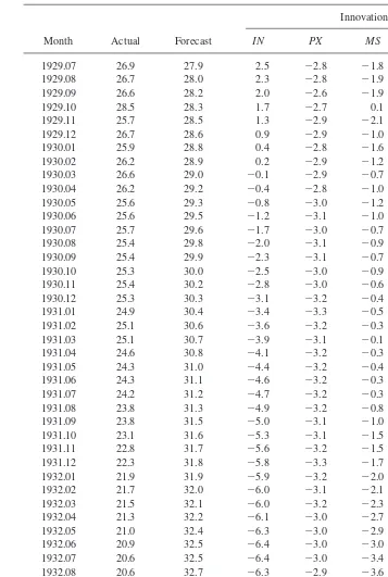
Table 5 examines the historical decomposition of the price time series. As in the case of the output series, at the beginning of the Great Depression, actual price level exceeded the forecast level. The higher than expected price level is explained by positive shocks in output, prices and, to a small extent, by the deposits of failed banks. Negative shocks to money supply initiated the fall in prices, and these shocks lasted until August 1930. By this time, negative shocks to output, which began to affect prices adversely from February 1930, were becoming increasingly more important and remained strong during the rest of the period under study. Own positive price shocks were initially responsible for higher than expected price levels but gradually became weaker, and by November 1930, negative own shocks started to affect prices for the remainder of the period. The fall in prices was exacerbated by negative shocks in money supply and deposits of failed banks beginning in January 1932 and June 1931, respectively. The negative impact of failed banks on prices exceeded own shocks in the last month under study. These results suggest that bank failures not only impacted output but also prices; indeed, prices were affected earlier than output by bank failures during the Great Depression. Consistent with discussion of the sequence of events during the Great Depression in Friedman and Schwartz (1963, p. 355), as bank runs took place, banks sold off assets to pay depositors’ claims, but this caused asset values and the general price level to fall sharply. Finally, shocks from the liabilities of failed businesses, again, had little impact.
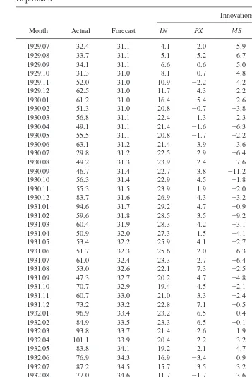
Table 6 contains the results for the money supply time series. Here we see that the actual money supply was less than the expected money supply throughout the entire period under study. This difference gradually increased over time and, by March 1933, reached 30%, which continued in the months after the bank holiday. This persistent and significant shortage implies that the prevailing levels of output and prices required a far greater supply of money than was being provided by the central bank. These results strongly support the monetarist views of Friedman and Schwartz (1963) and others that money supply shortages over an extended period of time were a key factor in explaining the collapse of output and prices in the Great Depression. According to Friedman and Schwartz (1963, p. 353), bank failures during the Great Depression caused deposits to be much less desirable to the public and led to a sharp decline in money supply (i.e., currency and deposits). The Federal Reserve viewed the bank failures as a result of poor manage-ment and the excesses of the past, rather than as causes of the financial and economic collapse process. In other words, they viewed the banking difficulties as separate from money and credit effects. Neither the liabilities of failed businesses nor the deposits of failed banks appeared to affect the decline in the money supply.
Table 7 presents decomposition results for the liabilities of failed businesses. Initially, the actual liabilities of failed businesses were close to their forecast. In the last few months of 1929, the gap increased and later reached differentials of two to three times in some months. The difference was explained by positive shocks from output, and these shocks
Table 5. Historical Decomposition of Wholesale Price Index Series During the Great
Table 6. Historical Decomposition of Money Supply Series During the Great Depressiona
Table 7. Historical Decomposition of Liabilities of Failed Businesses Series During the Great 1932.03 93.8 33.7 21.4 2.6 1.9 26.1 8.1 1932.04 101.1 33.9 20.4 2.2 3.2 34.9 6.6 1932.05 83.8 34.1 19.2 2.1 4.7 16.6 7.2 1932.06 76.9 34.3 16.9 23.4 0.9 20.1 8.1 1932.07 87.2 34.5 15.7 3.5 3.2 21.7 8.5 1932.08 77.0 34.6 11.7 21.7 3.6 20.2 8.7
became increasingly more important over time. In other words, increased business failures were a response to falling output. The rise in the liabilities of failed businesses were worsened by their own shocks as well as by shocks from the deposits of failed banks, the latter of which became the dominant force near the end of the period. Consistent with our earlier findings in Table 4, we infer here that bank failures contributed to increased numbers of business failures, especially when bank failure became a chronic condition in the banking system.
Lastly, Table 8 shows the results of the historical decomposition of the deposits of failed banks. Prior to the bank holiday, actual figures generally exceeded the forecasted deposits of failed banks and, in many cases, this difference was very large in magnitude. For example, in March 1933, the actual deposits of failed banks surged to $3,276.7 million or 73 times expected deposits of $44.9 million. About 82% of the $3,231.8 million discrep-ancy is explained by own shocks, while shocks to output, prices, money supply, and the liabilities of failed businesses explain 3.5%, 2.6%, 3.0%, and 8.8%, respectively.
V. Summary and Conclusions
To examine the nonmonetary effects of the financial crisis during the Great Depression, this paper employed vector autregression (VAR) for modeling the dynamic relationships between the real economy and the financial system. The results from the historical decomposition of time series of industrial production, prices, money supply, liabilities of failed businesses, and the deposits of failed banks generated from the VAR model suggest that the deposits of failed banks did not play an important role in explaining the fall in output during the first two years of the Great Depression. However, when bank failures occurred for an extended period of time, the repeated shocks from the banking sector eventually began to adversely affect the real economy. Indeed, by the end of the depression, persistent bank failure shocks, in combination with a surge in failures in the latter part of this period of banking industry distress, became an important source of the fall in output, prices, and money supply, not to mention business activity. Thus, we conclude thatchronicbank failures coupled with threshold failure effects can have deep and pervasive effects on the economy.
An important policy implication of our findings is that, when bank failures are short-term in nature, they have little impact on the economy. However, chronic bank failures that are cumulatively substantial, as well as sudden surges of large numbers of bank failures, necessitate the use of government intervention to stabilize the banking system and assure that the process of financial intermediation fosters the provision of credit services in the economy. Relatedly, although the continuing deregulation of banks in the United States (as well as in other major industrial countries) since the early 1980s tends to increase competition and bank failure risk, our results imply that the credit hypothesis is a long-run, rather than short-run, concern in this deregulation process. For this reason, intermittent bank failures stemming from deregulation should not affect the real economy unless they become chronic and substantial in nature.
Table 8. Historical Decomposition of Deposits of Failed Banks Series During the Great 1929.11 22.3 14.5 23.1 211.7 2152.6 35.7 113.3 1929.12 15.5 14.8 46.9 256.7 251.1 243.9 2196.8 1930.01 26.5 15.1 53.7 217.4 253.5 15.2 13.4 1930.02 32.4 15.4 47.4 27.0 98.3 24.2 2151.4 1930.03 23.2 15.7 39.2 36.9 2108.5 233.8 73.6 1930.04 31.9 16.1 20.2 223.3 22.5 240.4 61.9 1930.05 19.4 16.5 216.3 26.7 58.6 2109.5 43.3 1930.06 57.9 16.9 13.1 15.3 9.7 2137.4 140.4 1930.07 29.8 17.3 53.9 218.0 123.8 211.7 2135.6 1930.08 22.8 17.7 79.6 53.0 268.8 34.0 292.6 1930.09 21.6 18.2 90.0 25.4 46.9 242.6 2116.4 1930.10 19.7 18.7 111.2 234.9 227.3 221.9 226.2 1930.11 179.9 19.3 85.5 15.8 24.7 106.0 271.4 1930.12 372.1 19.8 89.4 30.6 270.9 140.1 163.1 1931.01 75.7 20.5 86.7 213.0 249.8 19.2 12.1 1931.02 34.2 21.1 127.2 235.3 12.5 41.9 2133.3 1931.03 34.3 21.8 106.9 8. 225.5 51.0 2127.9 1931.04 41.7 22.5 109.3 24.6 246.3 20.3 268.2 1931.05 43.2 23.2 110.3 27.5 216.8 218.5 282.5 1931.06 190.5 24.0 86.3 47.9 19.1 2149.8 162.9 1931.07 40.8 24.8 107.5 75.8 27.9 2155.8 23.6 1931.08 180.0 25.6 94.3 84.2 224.8 20.8 1.6 1931.09 233.5 26.4 102.4 21.1 20.6 140.4 277.4 1931.10 471.4 27.3 91.1 40.1 26.5 9.5 277.0 1931.11 67.9 28.1 98.4 19.9 62.2 4.5 2145.3 1931.12 277.1 29.1 128.7 227.8 13.3 148.6 214.9 1932.01 218.9 30.0 140.8 216.9 0.9 27.6 36.5 1932.02 51.7 30.9 94.5 231.4 26.7 287.0 51.4 1932.03 10.9 31.9 77.5 32.5 11.1 8.3 2150.5 1932.04 31.6 32.9 51.2 238.9 31.7 2113.8 68.5 1932.05 34.4 33.9 62.7 25.4 1.2 272.0 217.0 1932.06 132.7 35.0 39.8 5.9 210.2 53.8 8.4 1932.07 48.7 36.0 75.0 40.4 221.5 2108.7 27.5 1932.08 29.5 37.1 92.0 9.6 5.8 2116.1 1.1 1932.09 13.5 38.2 65.2 29.7 215.4 211.9 292.4 1932.10 10.1 39.3 56.3 27.7 6.3 42.8 2152.2 1932.11 43.3 40.4 70.4 215.9 20.7 47.4 2119.5 1932.12 70.9 41.5 77.1 59.6 24.2 83.2 2186.3 1933.01 133.1 42.6 67.7 25.2 7.4 112.9 2122.8 1933.02 62.2 43.7 96.5 31.3 233.0 130.6 2206.9 1933.03 3276.7 44.9 114.1 85.5 96.8 284.2 2651.3 1933.04 18.8 46.0 59.4 5.8 111.6 210.7 2414.7 1933.05 32.7 47.2 18.4 37.6 214.1 221.7 234.7 1933.06 21.9 48.4 34.2 210.7 29.2 25.5 266.3 1933.07 10.7 49.6 32.8 26.9 27.3 68.8 2126.2 1933.08 18.9 50.8 212.7 237.6 45.6 25.0 252.1
a
References
Akaike, H. 1973. Information theory and the extension of the maximum likelihood principle. In Proceedings of the2nd International Symposium on Information Theory(B.N. Petrov and F. Csaki, eds.). Budapest, 267–281.
Bernanke, B. S. June, 1983. Nonmonetary effects of the financial crisis in the propagation of the Great Depression.American Economic Review73(3):257–276.
Bernanke, B. S., and James, H. 1991. The gold standard, deflation, and financial crises in the Great Depression: An international comparison. In Financial Markets and Financial Crises (R. G. Hubbard, ed.). Chicago: University of Chicago Press, Inc.
Bernanke, B. S., and Carey, K. 1994. Nominal wage stickiness and aggregate supply in the Great Depression. Princeton: Princeton University Press.
Bernanke, B. S. February, 1995. The macroeconomics of the Great Depression: A comparative approach.Journal of Money, Credit, and Banking27(1):1–28.
Bernanke, B. S., and Gertler, M. L. 1987. Banking and macroeconomic equilibrium. In New Approaches to Monetary Economics (W. A. Barnett and K. Singleton, eds.). New York: Cambridge University Press, pp. 89–111.
Best, R., and Zhang, H. September, 1993. Alternative information sources and the information content of bank loans.Journal of Finance48(4):1507–1522.
Boyd, J. H., and Graham, S. L. 1996. Consolidation in U.S. banking: Implications for efficiency and risk. Working Paper 572. Federal Reserve Bank of Minneapolis.
Calomiris, C. W., Hubbard, G. R., and Stock, J. H. 1986. The farm credit crisis and public policy.
Brookings Papers on Economic Activity:441–479.
Diamond, D. W., and Dybvig, P. H. June, 1983. Bank runs, deposit insurance and liquidity.Journal of Political Economy91(3):410–419.
Dickey, D., and Fuller, W. A. June, 1979. Distribution of the estimators for autoregressive time series with a unit root.Journal of the American Statistical Association74(3):427–431. Engle, R. F., and Granger C. W. J. March, 1987. Cointegration and error-correction: Representation,
estimation and testing.Econometrica55(2):251–276.
Friedman, M., and Schwartz, A. J. 1963.A Monetary History of the United States, 1867–1960. Princeton: Princeton University Press.
Fuller, W. A. 1976.Introduction to Statistical Time Series. New York: Wiley.
Gertler, M. August, 1988. Financial structure and aggregate economic activity: An overview.
Journal of Money, Credit, and Banking20(3):559–588.
Gilbert, A. R., and Kochin, L. A. December, 1989. Local economic effects of bank failures.Journal of Financial Services Research3(4):333–345.
Gurley, J. G. and E. S. Shaw. September, 1955. Financial aspects of economic development. American Economic Review 45(4):515–538.
Hafer, R., and Sheehan, R. January, 1991. Policy inference using VAR models.Economic Inquiry
29(1):44–52.
Haubrich, J. G. March, 1990. Nonmonetary effects of financial crisis: Lessons from the Great Depression in Canada.Journal of Monetary Economics25(2):223–252.
Johansen, S. June/September, 1988. Statistical analysis of cointegration vectors.Journal of Eco-nomic Dynamics and Control12(2 and 3):231–254.
Johansen, S. November, 1991. Estimation and hypothesis testing of cointegration vectors in Gaussian vector autoregressive models.Econometrica59(6):1551–1580.
Johansen, S. 1992. Determination of the cointegration rank in the presence of a linear trend. Oxford Bulletin of Economics and Statistics 54:383–397.
InEconometric Decision Models: New Methods of Modeling and Applications(J. Gruber, ed.). Berlin: Springs Verlag.
Kaufman, G. G. April, 1994. Bank contagion: A review of the theory and evidence.Journal of Financial Services Research8(2):123–150.
Kaufman, G. G. 1996. Bank failures, systematic risk, and bank regulation. Working Paper WP-96-1. Federal Reserve Bank of Chicago.
King, R. G., Plosser, C. I., Stock, J. H., and Watson, M. W. June, 1991. Stochastic trends and economic fluctuations.American Economic Review81(4):819–840.
King, S. 1985. Monetary transmission: Through bank loans or bank liabilities? Mimeograph. Stanford University.
Kugler, P., and Lenz, C. February, 1993. Multivariate cointegration analysis and the long-run validity of PPP.The Review of Economics and Statistics75(1):180–184.
Levine, R. June, 1997. Financial development and economic growth: Views and agenda.Journal of Economic Literature35(2):688–726.
Mason, J. R. 1998. Evidence on indirect bankruptcy costs: The opportunity cost of capital, liquidation rates, and the value of intertemporal asset storage across the business cycle. Working Paper. Office of the Comptroller of the Currency.
Moore, R. R. December. Government guarantees and banking: Evidence from the Mexican peso crisis.Financial Industry Studies, Federal Reserve Bank of Dallas:13–21.
Phillips, P., and Perron, P. June, 1988. Testing for unit roots in time series.Biometrika75(2):334–346. Samolyk, K. A. Quarter 2, 1990. In search of the elusive credit view: Testing for a credit channel in modern Great Britain.Economic Review, Federal Reserve Bank of Cleveland 26(2):16–28. Schwarz, G. March, 1978. Estimating the dimension of a model.Annals of Statistics6(3):461–464. Wheelock, D. C. March/April 1995. Regulation, market structure, and the bank failures of the Great
Depression.Review, Federal Reserve Bank of St. Louis:27–38.
Appendix
Unit Root Tests
For a time series,x, the Augmented Dickey-Fuller test is thetstatistic associated withain the following equation:Dxt5m1axt211¥ni51biDxt2i1et, whereDxt2iis the first difference
of xt21, and nis the number of its lag, so that et is white noise. The critical values of
Dickey-Fuller statistics were provided by Dickey and Fuller (1979) and Fuller (1976). Phillips and Perron (1988) nonparametricZaandZtfor any variable,x, are defined as: