www.elsevier.com / locate / econbase
Productivity slowdown due to scarcity of capital to scrap in a
putty-clay model
*
Thomas Lindh
Department of Economics, Uppsala University, Box 513, 751 20 Uppsala, Sweden
Received 19 August 1999; accepted 7 March 2000
Abstract
The conditions for a productivity slowdown to take place simultaneously with accelerated technical change are investigated in a simple putty-clay macro model of the Johansen type. A capacity distribution such that the resulting supply curve is concave at the scrapping margin means a high likelihood of a reversed relation. The relation between growth rates of wages and output is crucially dependent on the tail elasticity of the capacity distribution. The need in a putty-clay economy to scrap in order to transfer labor to new investment is the key mechanism. The model emphasizes the decisive role of past investment in shaping the current relation between technical change and productivity growth. 2000 Elsevier Science S.A. All rights reserved.
Keywords: Productivity slowdown; Putty-clay; Capacity distribution
JEL classification: O41
1. Introduction
If production is characterized by putty-clay technology and production units on the verge of scrapping are relatively scarce, relatively few low-productivity jobs are replaced by new high-productivity jobs. Productivity growth slows down even if the rate of technical change in best-practice units remains at a high level. The productivity slowdown in the late 1960s or somewhat later, experienced by almost all industrialized nations, could have to some extent depended on investment slumps in the 1930s and 1940s. Many other explanations have been offered, most often the rise in energy prices in 1973, but declining knowledge production, slower rates of increase in labor skill, declining investment rates, shifts towards service production, and increasing government sectors and distorting taxes have also been put forward as causes; cf. Fischer (1988). But the productivity
*Tel.:146-18-471-1103; fax: 146-18-471-1478. E-mail address: [email protected] (T. Lindh).
226 T. Lindh / Economics Letters 69 (2000) 225 –233
slowdown still remains largely a puzzle and none of the possible causes has been generally accepted to explain more than minor parts of the slowdown. Recently, the age of the capital stock has received renewed attention as part of the explanation; see Wolff (1996). The work of Davis and Haltiwanger (1992) and their followers on gross job flows has also revived interest in putty-clay models, since the actual gross flows observed in the economy are hard to reconcile with conventional aggregate production functions.
The point made in this paper is that the form of the capacity distribution in itself influences how technical change translates into productivity growth, and may temporarily make the relation negative. A putty-clay model, where capital can be substituted for labor only prior to the actual investment, provides an analytical tool for the hypothesis that scarce capital to scrap may cause a productivity slowdown. The aim here is, however, only to make a precise and simple statement of a mechanism that seems to be generally overlooked in the literature.
The basic idea is a variation on the old theme of echo effects first put forward by Karl Marx. Einarsen (1938) contains much of the early history. Salter (1960, 1965) discussed the importance of the capacity structure extensively in a vintage context. Two contributions by Benhabib and Rustichini (1991, 1993) investigates echo effects both theoretically and empirically with models where capital equipment is subject to fixed depreciation patterns. The model used here entails endogenous obsolescence driven by exogenous technical change in a Johansen (1972)-type short-run macro production function with a simple (one variable factor) version as formulated by Pomansky and Trofimov (1990). Throughout this paper, productivity refers to labor productivity since a consistent capital aggregate independent of labor cannot be constructed in this type of model.
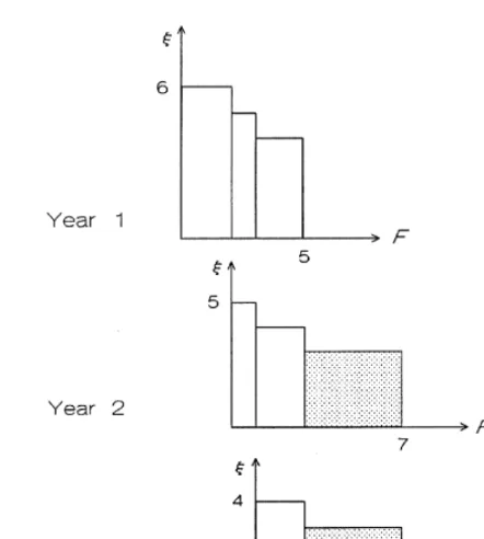
The essential mechanism of the model is illustrated in Fig. 1. The decrease in productivity growth is due to scarcity of old equipment, which cannot cover wage costs, and therefore only a small amount of labor is freed to be transferred to new equipment. By raising wages more than best-practice productivity increases, more labor could be released, but that would not be the optimal thing to do, since capital costs could not then be covered.
The paper is organized as follows. To save space, only a very simple version of the model is
1
presented. Section 2 develops the formal model of a putty-clay production structure. Section 3 treats the dynamics of the model, and Section 4 briefly discusses its empirical relevance. Section 5 summarizes the argument.
2. A putty-clay model
One homogeneous good is produced by labor, using capital equipment, heterogeneous over time but ´
homogeneous at the moment of installation. The good (and numeraire) can either be immediately consumed or frozen into capital equipment which is impossible to recover for consumption.
Let j denote labor input coefficients and c(j) the continuously differentiable density of the distribution of production capacity over input coefficients. Assume that all available labor, V, is allocated to maximize production. Then no production unit with higher input coefficient will be used before capacity with lower input coefficients is fully utilized.
1
Fig. 1. Labor input coefficients are measured on the vertical axis and accumulated output on the horizontal axis. Total labor is measured by the area of the bars. Each year the input requirements in best-practice technology decrease with unity (i.e. productivity growth accelerates from 0.33 to 0.5). Given that only units with the highest input coefficients are scrapped, the area of the new bar must equal that of the scrapped units. Hence average productivity growth decelerates (from 0.4 to 0.21) while productivity on the scrapping margin (equal to wages) accelerates (from 0.2 to 0.25).
Both the input coefficient and the capacity corresponding to a given production unit are fixed. To avoid dealing with changes in the interior of the support of the distribution I assume that all new production units will use a marginally lower input coefficient than any existing. Hence
R(V,t )
F(V,t)5
E
c(j)dj, (2.1)X(t )
where X(t) denotes the minimal input coefficient in existing production equipment and R(V,t) the maximal actually used at the current time t. Furthermore,
R(V,t )
V(t)5
E
jc(j)dj. (2.2)X(t )
Differentiate (2.1) and (2.2) w.r.t. V, subindexes denote partial derivatives:
1
]
FV5c(R)R and 1V 5Rc(R)RV⇒FV5 . (2.3)
228 T. Lindh / Economics Letters 69 (2000) 225 –233
Aggregate marginal productivity equals average productivity in the marginal production unit and, thus, the wage rate, a standard result for this type of model.
Differentiate (2.1) and (2.2) w.r.t. t. A dot over a variable denotes total time differentiation:
~ ~ ~
Ft1F VV 5 2c(X )X1c(R)(Rt1R V ),V
~ ~ ~
V5 2Xc(X )X1Rc(R)(Rt1R V ).V (2.4)
From (2.3) it follows that all terms involving the time derivative of V will cancel out in both equations. By definition, the flow of new output capacity at any given point in time is
Rt X
~ ]
S
]D
w(t)82c(X )X5 2Rc(R) ⇒Ft5w 12 (2.5)
X R
by using (2.4).
To simplify, V is henceforth assumed to be constant and equal to unity, and there is, therefore, no need to distinguish the total and partial time derivatives of F and R. Note, however, that this assumption is not needed for (2.5) to hold.
The capacity flow w and the minimal input coefficient X are determined by decisions of a representative firm. The firm chooses investment, k, and labor input flow,v, in order to maximize the
present value of its future profit flow from the investment. The ex ante production function
12a a
f(k,v,t)5u(t)k v (2.6)
is a constant returns to scale Cobb–Douglas function. Let r be the expected path of the interest rate and wv the expected path of wage increases. The firm takes w, current wages, as given and solves the problem
where l is the expected economic life of the investment. Expectations of strictly rising wages will then imply a finite l and also an expected period of usage that is connected.
The present value function may be convex in k and v due to the dependency of a consistent
expectation of l on the capital / labor ratio chosen, so a unique maximum cannot be guaranteed in
2
general. Here it is assumed that f and expectations have the properties needed for uniqueness. To simplify further, write
and assume these expectation-dependent variables can be treated as fixed (see Section 4 for a
2
justification of this drastic assumption). The first-order conditions for maximization can then be
The firm also has to decide whether to continue or discontinue operations on existing units. Since there is no alternative use of equipment and the capacity density is continuous, the marginal unit can exactly cover its costs, i.e.
1
]
w5 5Fv. (2.10)
R
Under these assumptions it turns out that the ratio of X to R will be constant, since (2.9) and (2.10) ensure this ratio is proportional to D/W. Hence the change in output only varies with the flow of new capacity.
3. Dynamics of the model
In this section the relation between capacity structure and productivity growth is derived. With V fixed the proportional rate of change in labor productivity is identical to the proportional rate of change in aggregate production. So the percentage change in productivity growth is by definition
2 2 2
ˆ ~
F5F2F (3.1)
where one hat indicates the logarithmic differential operator w.r.t. t, and two hats the repeated application of that operator. The growth rate of output is positive by the assumptions made, so the sign of the first term will be sufficient, although not necessary, to tell whether productivity growth slows down or not. Define the elasticity of the capacity density at input coefficient j as
c9(j)j ]]]
e(j)8 . (3.2)
c(j)
The first term on the RHS of (3.1) can be related to wage changes. By (2.5) we have
2
2 X
~ ˆ
S
]D
ˆF5w1 12 5w,
R
since X /R is constant. From the definition of capacity flow in (2.5) it follows that
230 T. Lindh / Economics Letters 69 (2000) 225 –233
3
Wage changes can be shown to be proportional to changes inu, the technique factor, and so from (3.3) it follows that productivity will decelerate for certain values of e(R) even if wages, or equivalently technical change, accelerate.
2 2
ˆˆ ˆ
Proposition 1. u,F and e(R)$ 21 implies F#0.
Proof. By inspection of (3.1) and (3.3). h
Thus, even as technical change accelerates, productivity may decelerate. A short run schedule of supply, that is concave at the margin, would be even more sufficient, since
Proposition 2. The price schedule of supply is concave at the margin if and only if e(R)$0.
Proof. LetC(j) be production as a function of the highest input coefficient used. Then
C9(j)5c(j) andC0(j)5c9(j).
InvertC(j) to obtain the price schedule of supply j(C) in terms of labor units. It follows that
e(j)
1 C0
] ]] ]]]
j9(C)5C9 andj0(C)5 2 35 2 2, (C9) jc(j)
proving this assertion for all open sets where C9(j)±0. Due to our assumption of a connected
support of c it therefore holds for X#j #R. h
4
Note that in Fig. 1 the bars depict a reversed supply schedule, which when smoothed will be concave at the marginal unit.
The elasticity e(R) is positive whenever c(R) is increasing, e.g. if past investment has been insufficient to raise capacity flow at the same rate as input coefficients decreased. In steady state with positive growth, e(R)5 22 everywhere (Pomansky and Trofimov, 1990).
It can be shown that the steady-state structure is actually a boundary case, since if e(R) is only slightly greater than 22 and the capacity distribution otherwise has the steady-state elasticity, except for a small neighborhood of R, there could be deceleration even for a constant rate of technical change.
Generalizations of the assumptions of course modify these conclusions, but the essential thrust of
5
the argument is preserved. The effects of some generalizations are summarized below.
An elasticity of substitution in the ex ante production function below unity would tend to slow down productivity growth. Intuitively the labor restriction is restricting growth more seriously when labor is harder to substitute for.
A decreasing ratio W/D will make a slowdown likely whene(R). 21, because the difference in
3
From the first expression in the first-order conditions (2.9) and the assumption of fixed expectations it follows that
ˆ ˆ ˆ ˆ
Accumulating supply from the least efficient to most efficient units instead of the other way around. 5
growth rates in W and D is then negative and the relative gap in input coefficients will decrease. This would be consistent with increasing scrapping rates and a relatively abundant supply of labor at the same time as quasi-rents diminish. This could be the case in the later stages of a slowdown due to scarcity of scrapping and would hence tend to prolong the time to recovery.
Probably, growth in labor supply will accelerate labor productivity growth, but there are also mechanisms working in the other direction so the contribution cannot in general be determined.
4. Empirical relevance
The real world is of course not strictly putty-clay. On the other hand, old capital is not a perfect substitute for new capital either, and labor can be reallocated without scrapping only to the extent that input coefficients in older equipment are flexible. Different capital items will have very varying lengths of life, but complementarities among items could still make it likely that much of the scrapping in any given year is dominated by units of equipment and replacements of short-lived components originally installed within a fairly narrow period of time.
Is there then any empirical evidence in favor of putty-clay effects from an irregular capacity distribution? Benhabib and Rustichini (1993) and Biørn and Frenger (1987) estimate putty-clay vintage models on aggregate data (1929–1988 and 1964–1983, respectively) with these results. There is more evidence pointing to the possibility of putty-clay effects. Space permits us to mention only some of it.
6
There is micro evidence from surveys of metalworking equipment in the United States that substantial parts of the equipment installed in the late 1930s were in operation up to the 1970s and that the metalworking machinery as an aggregate was aging fast in the beginning of the 1930s and the 1960s.
As can be deduced from Eq. (3.3) the variation in wage growth and average labor productivity would tend to move out of phase shortly after a period with scarce capital to scrap. This is evident in data from the 1970s in Sweden, where wage costs surged upwards in the mid 1970s while at the same time productivity growth fell and even became negative. Similar developments can be documented for many other countries. In the U.S. data a similar desynchronization takes place somewhat earlier in the 1960s and recurs later in the 1980s.
There is a well-established empirical correlation between investment and growth. In this model, from (2.5) and the first-order conditions (2.9) it can be derived that
12a(W/D )
]]]]
Ft5 k. (4.1)
D(12a)
A simple regression of the labor corrected change of GDP (F ) on investment (k) using 117 years oft Swedish data yields a highly significant coefficient of about 0.08, which is consistent with reasonable values of the parameters. Hence, conditional on the putty-clay hypothesis, in the medium run it seems no serious empirical restriction to add the Cobb–Douglas and fixed expectation assumption.
6
232 T. Lindh / Economics Letters 69 (2000) 225 –233
Of course, the capital structure may also be such that it enhances productivity acceleration and compensates for retardation in technical change. This other side of the coin is thus consistent with the hypothesis that the echoes from high investment activity in the 60s reached us in the 90s. However, it is hard to find data on the vintage structure of capital to verify such an hypothesis. Ma and Lau (1994) develop the theoretical possibility to recreate the distribution from aggregate profit function data which may be helpful in view of the scarcity of direct data.
5. Conclusions
In a simple model with putty-clay capital, acceleration in the rate of technical change can take place at the same time as a deceleration in the growth rate of aggregate productivity. An elasticity of the capacity density that is not too negative, or equivalently a supply schedule that is not too convex, will guarantee this under the assumptions made here. It is worth pointing out two features of the model. First, it may very well take a long time — on the order of centuries — before the final effects of technical change are reached, presumably long after the equipment implementing it was scrapped, because price responses to imbalances in the capacity distribution will result in further imbalances in the structure echoing down in time. Second, it bears stressing that the slowdown in the model is not due to any economic inefficiency. On the contrary, with given price expectations, the representative firm acts optimally and a social planner would face the same mechanisms. Moreover, the results are derived under the assumption of full employment and immediate reallocation of labor.
Acknowledgements
I thank A.B. Pomansky and G.Y. Trofimov for the suggestion to use the Johansen model. I have also benefited from comments by L. Lau and S. Lundgren. Financial support from Jan Wallanders och Tom Hedelius’ stiftelse is gratefully acknowledged.
References
Fourteenth American Machinist Inventory, 1989. Penton, Cleveland.
Benhabib, J., Rustichini, A., 1993. A vintage capital model of investment and growth: theory and evidence. In: Becker, R., Boldrin, M., Jones, R., Thompson, W. (Eds.), General Equilibrium Growth and Trade II: The Legacy of Lionel Mckenzie. Academic Press, San Diego.
Benhabib, J., Rustichini, A., 1991. Vintage capital, investment, and growth. Journal of Economic Theory 55, 323–339. Biørn, E., Frenger, P., 1987. Expectations, substitution, and scrapping in a putty-clay model. Discussion Paper No. 17,
Central Bureau of Statistics, Norway.
Bliss, C., 1968. On putty-clay. Review of Economic Studies 5, 105–132.
Davis, S.J., Haltiwanger, J.C., 1992. Gross job creation, gross job destruction, and employment reallocation. Quarterly Journal of Economics 107 (3), 819–863.
Einarsen, J., 1938. Reinvestment cycles and their manifestation in the Norwegian shipping industry. Publication No. 14, University Institute of Economics, Oslo.
Ma, B.K., Lau, L.J., 1994. The short-run aggregate profit function and the capacity distribution. Scandinavian Journal 96 (2), 201–218.
Lindh, T., 1992. Essays on expectations in economic theory. Acta Universitatis Upsaliensis, Studia Oeconomica Upsaliensia 21. Alinqvist & Wiksell International, Stockholm.
Pomansky, A.B., Trofimov, G.Yu., 1990. Model of the localized technical progress and structural shifts in the industry (transl. of Russian title). Ekonomika i Matematicheskie Metody 26 (5).
Salter, W.E.G., 1960. Productivity and Technical Change. Cambridge University Press.
Salter, W.E.G., 1965. Productivity growth and accumulation as historical processes. In: Robinson, E.A.G. (Ed.), Problems in Economic Development. MacMillan, London, pp. 266–294.