Conference paper

(1)

STUDY OF TEMPORAL VARIATION OF VEGETATION INDICES AND PHENOLOGY

OF TROPICAL DECIDUOUS BROADLEAF FOREST IN EASTERN INDIA

Udit Gupta

Indian School of Mines Dhanbad, India, uditguptaism@gmail.com

Commission VIII, WG VIII/8

KEY WORDS:Vegetation, Forestry, Identification, Monitoring, Satellite, Multitemporal

ABSTRACT:

In the recent years study of vegetation variation has taken significance as a quintessential part of a bigger research agenda of climate change. This study has attempted to (a) Analyse the inter-annual and seasonal variation of vegetation (b) Observe the variation in phenological transition dates of tropical deciduous broadleaf forest (DBF) in Eastern India from 2003 to 2012. The study was conducted on 1500 sq. km area of dense forest in the districts of West Singhbhum and Sundargarh. MODIS EVI data of 250 meter resolution was used. Land cover mask was used to study only the DBF pixels. Least squares convolution method proposed by Savitzky and Golay was used for noise reduction and smoothing. For the determination of phenological parameters iterative Savitzky-Golay method followed by threshold method was used in TIMESAT software. The results showed that (i) EVI varied between 0.41 in early April and 0.71 in mid October (ii) The overall trend was decreasing with a slope of 0.0022, representing a degradation trend (iii) EVI of summer season was found to be more stable than of rainy and winter season (iv) Summer and rainy months showed a decreasing trend whereas the winter months showed an overall increase (v) Day of start of season varied between 2nd_{May and 20}th_{June whereas the day of end of season varied between 1}st_{February and 7}th_{March (vi) Length of season was longest} for 2007 at 302 days and shortest for 2010 at 235 days and showed an overall decreasing trend.

1. INTRODUCTION

Vegetation is an important component in the biogeochemical cycle because of its relationship and crucial ability to affect the other components and the climate as a whole. In turn, climate change also affects vegetation dynamics, phenology and ecophysiology (Theurillat and Guisan, 2001). In the recent years study of vegetation dynamics has taken significance as a quintessential part of a bigger research agenda of climate change (Xin, Xu and Zheng, 2008).

Satellite measurements have been frequently used for vegetation monitoring at varying spatial and temporal scales (e.g., Myneni et al., 1997).The low temporal resolution is a major barrier in analyzing dynamic variation. However, long time series can be extracted and observed for long term trends in vegetation suitably. Recently, due to the large availability of free to cheap satellite data sources like Moderate Resolution Imaging Spectroradiometer (MODIS) and Advanced Very High Resolution Radiometer (AVHRR), this application of remote sensing data has been extended to the study of phenology as well (Wu et al., 2010, Zhang et al., 2003). Traditionally Normalised Difference Vegetation Index (NDVI) has been used in studying spatial and temporal vegetation variation (Zhang et al., 2014) and phenology (Jönsson et al., 2010). This study uses Enhanced vegetation index (EVI) which was developed to incorporate atmospheric and background corrections and is much more sensitive to high biomass areas (Huete et al., 2002).

In India, there is a lack of scientific data on extent, type and the condition of tropical forests (Roy and Joshi 2002). Recently, GIMMS and MODIS data was used to extract phenological parameters across the country (Jeganathan and Nishant, 2013).

This study aims to (a) Analyse the inter-annual and seasonal variation of vegetation (b) Observe the variation in seasonality metrics of tropical deciduous broadleaf forest (DBF) in Eastern India from 2003 to 2012.

2. STUDY AREA

The study area is located in West Singhbhum district of Jharkhand and Sundargarh district of Odisha. The 1500 square kilometers area is centered at the coordinate 22.190o N 85.206o E. The area is chosen because a high percentage of the area is under deciduous broadleaf forest (28.6 %). Sal (Shorea robusta) is the most important tree in the area. The forest area in the West Singhbhum district is called Sarandha forest. The fauna reported in this forest are Indian elephant, leopard, sloth bear, wild boar, barking deer, langur, etc (Saranda Development Plan, 2014). This entire Saranda forest division is notified as core area of Singhbhum Elephant Reserve. The forests are home to around 36500 tribals dominantly belonging to Ho tribes. The sal occupies a central place in the lives of these tribals. The sustenance of this tribal population is intricately linked with the health of these forests (Dash, 2006). The area also contains 25% of the known iron ore deposits in the country and hence is a major centre of iron ore mining in the country. (About Saranda Development Plan, 2014). The region experiences three distinct seasons namely summer (March to June), monsoon (July-September) and winter (October to February) (Climate in Odisha (Orissa), 2014).

(a)

The International Archives of the Photogrammetry, Remote Sensing and Spatial Information Sciences, Volume XL-8, 2014 ISPRS Technical Commission VIII Symposium, 09 – 12 December 2014, Hyderabad, India

This contribution has been peer-reviewed.

(2)

(b)

3. Materials and Methods

3.1 Materials

MODIS1_{(or Moderate Resolution Imaging Spectroradiometer)} Vegetation Index data of 250 metres spatial resolution and recorded every 16 days was used. Abbreviated as MYD13Q1, the data set of MYD13Q1 containing Enhanced Vegetation Index (EVI) was extracted. Blue, red, and near-infrared reflectances, centered at 469-nanometers, 645-nanometers, and 858-nanometers, respectively, are used to determine the vegetation index. A land cover mask of MODIS land cover product (MOD11A2) of 500 metres spatial resolution is applied to analyse only the pixels representing deciduous broadleaf forest. This step reduced the interference due to the pixels representing other land cover classes. TIMESAT software was used to observe and indentify trends in seasonal vegetation development (Jönsson & Eklundh, 2004).

3.2 Quality

The MODIS EVI data (MYD13Q1) used provides 2 generic quality assurance (QA) bits for every pixel. The quality of the data was controlled by removing cloudy and corrupted pixels through these QA bits. The pixels that passed the quality filters were found to have considerable noise. EVI data was filtered and smoothed for denoising processing using a Savitzky-Golay smoothing filter (Savitzky and Golay, 1964). Proposed by Savitzky and Golay in 1964 this data smoothing method is based on local least-squares polynomial approximation. The data obtained after the operation of Savitzky-Golay filter is used to identify temporal trends in monthly, seasonal and inter-annual vegetation variation. To identify whether the long term trend is decreasing or increasing in nature, linear regression is performed.

3.3 Extraction of seasonality parameters

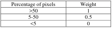
As an added measure to control quality of the data, a weighting system is used. This step takes into consideration the percentage of pixels that pass the generic quality assurance (QA) filter that is associated with all MODIS data. Table 1 describes the weighting scheme. After applying the aforementioned Savitzky-Golay method to the raw weighted data, seasonality parameters were determined by threshold method.

Percentage of pixels Weight

>50 1

5-50 0.5

<5 0

Table 1: Weighting scheme

The seasonality parameters determined are End of Season (EOS), Start of Season (SOS) and Length of Season (LOS). Different methods have been applied for indentifying start and end of season including land cover specific thresholds (Chen et al., 2000), absolute thresholds (Lloyd, 1990) and a percent of seasonal amplitude in TIMESAT (Jönsson and Eklundh, 2004). A threshold of 30 % of the seasonal amplitude was found to perform favorably in this case.

4. Results

4.1 Monthly variation

The average variation of EVI in a year is obtained by averaging the EVI for a fixed date every year. This is possible because the MODIS Terra satellite records the EVI data at almost the same day of every year. The plot obtained is depicted in Figure 2.The base value of EVI is 0.41 which represents a thick forest cover and ground foliage all round the year. EVI decreases sharply from the start of the year till middle of April after which it stabilizes near the base value. In the month of July, with the onset of monsoon the EVI rises sharply till a peak is reached at EVI value of 0.71 in middle of October.

Figure 2. Monthly Variation of EVI

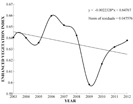
4.2 Inter Annual Variation

The enhanced vegetation index value over the whole study area is averaged for each year from 2003 to 2012. A linear fit curve is obtained through linear regression. The slope of the linear fit is negative with a value of 0.0022. This is representative of a degradation trend in vegetation across the study area. The higest annual EVI is observed in the year 2009. In the last three years however, the index value has increased significantly from the overall lowest value of 0.595 in 2009 to 0.64 in 2012.

(3)

Figure 3. Inter-Annual Variation of EVI

4.3 Seasonal Variation

The average value of each season is plotted in the figure 4. Summer months have a much lesser EVI than winter or monsoon months. The fluctations were observed to be less in summer months. Highest fluctuation was observed in the winter season. While summer and monsoon months showed an overall decreasing trend, the winter months showed an increasing trend.

Figure 4. Seasonal Variation of EVI

4.4 Start of Season (SOS)

The day of year (DOY) denoting start of growing season for every year is plotted in the figure 5. It is calculated by taking 30% of the seasonal amplitude as threshold. The SOS varied between 124th and 172th day of the year i.e. from start of May to third week of July. The decreasing linear fit represents that the start of season has been shifting towards an earlier day of the year.

4.5 End of Season (EOS)

The day of year (DOY) denoting end of growing season for every year is plotted in the figure 6. The EOS season or the day of leaf off varied from the 31st_{day to the 67}th_{day of the year} i.e. from the 31st January till the first week of March. The day of end of season is observed to have a slight shift towards the

start of the year. The fluctuations in EOS has been far less than observed in SOS with the years 2009, 2010 and 2011 having almost the same EOS.

Figure 5. Variation of DOY representing start of growing season.

.

Figure 6. Variation of DOY representing end of growing season.

4.6 Length of Season

Figure 7. Variation of length of growing season.

(4)

The length of growing season for every year is plotted in the figure 5. The length of season is calculated as difference between day of onset and day of offset of season. This duration of season is observed to show large fluctuations. The duration varied greatly between 232 days in to have 2007 to 300 days in 2010. The average duration of the season was 9 months. After the lowest value in 2010, the length however is observed to have increased steadily.

5. CONCLUSIONS

This study showed seasonal, annual and inter-annual vegetation variation (2002-12) of dry deciduous broadleaf forest in eastern India states. On studying the long term inter annual trends of EVI it is observed that the forests have undergone degradation. The observation of long term degradation raises a serious concern about the future of these pristine forests and more importantly about the life of tribal population and wildlife that these forests support. The phenological parameter represented by start of season, end of season and length of growing season are observed large variations. The phenological metrics extracted can be of much use to the scientific community and Singh, Assistant Professor, Department of Environment Science and Engineering, Indian School of Mines and Prof. Sue Grimmond, University of Reading for their support and guidance.

7. REFERENCES

Chen, X., Tan, Z., Schwartz, M. and Xu, C. (2000). Determining the growing season of land vegetation on the basis of plant phenology and satellite data in Northern China. International Journal of Biometeorology, 44(2), pp.97--101.

Dash, S. (2006). Naxal movement and state power. New Delhi: Sarup & Sons.

Measuring Vegetation (NDVI & EVI) (2014). [online] Available at: http://earthobservatory.nasa.gov/Features/Measur ingVegetation/measuring_vegetation_4.php [Accessed 7 Aug. 2014].

Huete, A., Didan, K., Miura, T., Rodriguez, E., Gao, X. and Ferreira, L. (2002). Overview of the radiometric and biophysical performance of the MODIS vegetation indices. Remote Sensing of Environment, 83(1-2), pp.195-213.

Jeganathan, C. and Nishant, N. (2013). Scrutinising MODIS and GIMMS Vegetation Indices for Extracting Growth Rhythm of Natural Vegetation in India. J Indian Soc Remote Sens, [online]42(2), pp.397-408. Available at: http://dx.doi.org/10.1007/s12524-013-0337-5 [Accessed 17 Jul. 2014].

Jönsson, A., Eklundh, L., Hellström, M., Bärring, L. and Jönsson, P. (2010). Annual changes in MODIS vegetation

indices of Swedish coniferous forests in relation to snow dynamics and tree phenology. Remote Sensing of Environment, 114(11), pp.2719-2730.

Jönsson, P. and Eklundh, L. (2002). Seasonality extraction by function fitting to time-series of satellite sensor data. Geoscience and Remote Sensing, IEEE Transactions on, 40(8), pp.1824--1832.

Jönsson, P. and Eklundh, L. (2004). TIMESAT- a program for analyzing time-series of satellite sensor data. Computers & Geosciences, 30(8), pp.833--845.

Lloyd, D. (1990). A phenological classification of terrestrial vegetation cover using shortwave vegetation index imagery. International Journal of Remote Sensing, 11(12), pp.2269-2279.

Myneni, R., Ramakrishna, R., Nemani, R. and Running, S. (1997). Estimation of global leaf area index and absorbed PAR using radiative transfer models. IEEE Transactions on Geoscience and Remote Sensing, 35(6), pp.1380--1393.

Orissatourism.org, (2014). Climate in Odisha (Orissa). [online] Available at: www.orissatourism.org/climate-in-orissa.html [Accessed 13 Aug. 2014].

Roy, P. and Joshi, P. (2002). Forest cover assessment in north-east India--the potential of temporal wide swath satellite sensor data (IRS-1C WiFS). International Journal of Remote Sensing, 23(22), pp.4881--4896.

Saranda.nic.in, (2014). Saranda Development Plan. [online] Available at: http://www.saranda.nic.in/index.html [Accessed 6 Jun. 2014].

Saranda.nic.in, (2014). About Saranda development plan. [online] Available at: http://www.saranda.nic.in/About_us.html [Accessed 7 Jun. 2014].

Savitzky, A. and Golay, M. (1964). Smoothing and differentiation of data by simplified least squares procedures. Analytical chemistry, 36(8), pp.1627--1639.

Theurillat, J. and Guisan, A. (2001). Potential impact of climate change on vegetation in the European Alps: a review. Climatic change, 50(1-2), pp.77--109.

Wu, W., Yang, P., Tang, H., Zhou, Q., Chen, Z. and Shibasaki, R. (2010). Characterizing spatial patterns of phenology in cropland of China based on remotely sensed data. Agricultural Sciences in China, 9(1), pp.101--112.

Xin, Z., Xu, J. and Zheng, W. (2008). Spatiotemporal variations of vegetation cover on the Chinese Loess Plateau (1981--2006): Impacts of climate changes and human activities. Science in China Series D: Earth Sciences, 51(1), pp.67--78.

Zhang, J., Zhang, L., Xu, C., Liu, W., Qi, Y. and Wo, X. (2014). Vegetation variation of mid-subtropical forest based on MODIS NDVI data. A case study of Jinggangshan City, Jiangxi Province. Acta Ecologica Sinica, 34(1), pp.7-12.

Zhang, X., Friedl, M., Schaaf, C., Strahler, A., Hodges, J., Gao, F., Reed, B. and Huete, A. (2003). Monitoring vegetation phenology using MODIS. Remote sensing of environment, 84(3), pp.471--475.