SPATIAL PATTERN OF TEMPORAL TREND OF CROP PHENOLOGY MATRICES OVER
INDIA USING TIMESERIES GIMMS NDVI DATA (1982-2006)
Abhishek Chakraborty*, Prabir Kumar Das, M V R Sesha Sai, G Behera
Agricultural Sciences & Applications Group, RS & GIS – Applications Area, National Remote Sensing Centre, Indian Space Research Organization, Hyderabad, India
KEY WORDS: Crop phenology, GIMMS NDVI, India, TIMESAT, Median trend
ABSTRACT:
NOAA-AVHRR bi-monthly NDVI data of 8×8 km for the period of 1982-2006 were used to analyze the trend of crop phenology matrices over Indian region. Time series principal component analysis of NDVI was performed to produce six calibration zones for fitting equations of temporal NDVI profile. Savitzky-Golay filter with different seasonality parameters, adaptation strengths and window sizes for different calibration zones were use to smoothen the NDVI profile. Three crop phenology matrices i.e. start of the growing season (SGS), Seasonal NDVI amplitude (AMP), Seasonally Integrated NDVI (SiNDVI) were extracted using TIMESAT software. Direction and magnitude of trends of these crop phenology matrices were analyzed at pixel level using Mann-Kendall test. Further the trends was assessed at meteorological subdivisional level using “Field significance test”. Significant advancement of SGS was observed over Punjab, Haryana, Marathwada, Vidarbha and Madhya Maharashtra where as delay was found over Rayalaseema, Coastal Andhra Pradesh, Bihar, Gangetic West Bengal and Sub-Himalayan West Bengal. North, West and central India covering Punjab, Haryana, West & East Uttar Pradesh, West & East Rajasthan, West & East Madhya Pradesh, Sourastra & Kutch, Rayalaseema, Marathwada, Vidarbha, Bihar and Sub-Himalayan West Bengal showed significant greening trend of kharif season. Most of the southern and eastern part of India covering Tamilnadu, South Interior Karnataka, Coastal Andhra Pradesh, Madhya Maharashtra, Gujarat region, Chhattisgarh, Jharkhand and Gangetic West Bengal showed significant browning trend during kharif season.
1. INTRODUCTION
Crop phenology is a study of recurring pattern of crop growth and development. Changes of crop phenology are recognized as being possibly the most important early indicator of impact of climate change on ecosystem. Variation of crop phenology has broad impacts on terrestrial ecosystems and human societies by altering global carbon, water and nitrogen cycles, crop production, duration of pollination season and distribution of diseases etc (Penuelas and Fiella, 2001; Soudani et al., 2008). Therefore, phenology has emerged recently as an important focus for ecological and climatic research (Menzel et al., 2001; Cleland et al., 2007). In situ observations, bioclimatic models and remote sensing constitute the three possible ways for monitoring the variations of vegetation phenological events (Schaber and Badech, 2003; Fisher et al., 2007). Remote sensing has the advantages of being the only way of sampling at low-cost with good temporal repeatability over large and inaccessible regions. Phenology from satellite observation is aggregate information at coarse spatial resolution that relates to the timing and rates of greening (growth) and browning (senescence), timing of maximum photosynthetic activities and duration of active growth phase at seasonal and inter annual time scales. Crop phenology is usually addressed through temporal monitoring of the normalized difference vegetation index (NDVI) time series, available since the launch of the earth observation satellites. The NDVI is calculated as the normalized difference between near-infrared and red bands, and quantifies the photosynthetic capacity of plant canopies, thus indicating the amount of vegetation present in one place. Time series NDVI data sets of NOAA/AVHRR, TERRA/MODIS and SPOT/VGT have been used in numerous studies to estimate the shift of vegetation phenological parameters and its relationships with different climatic and anthropogenic factors (Menzel et al., 2001; Zhou et al., 2001; Tao et al., 2006; Stockli and Vidale, 2004; Fontana et al., 2008; van Leeuwen et
al., 2010; Melezdez et al., 2010; Kariyeva et al., 2011). Most of these studies were carried out over North America, Europe, China. Central Asia, Sahel and Sudan region. The present study is an attempt to analyze the direction and magnitude of trend of few crop phenology matrices over Indian region.
2. METHODOLOGY 2.1 Study area
The study is carried out during kharif season over 25 meteorological subdivisions of India Meteorological Department (IMD) spread across 16 states of India (fig.1). The selected meteorological subdivisions have large contiguous areas of agricultural land and crop phenology could easily be indentified using coarse resolution time series satellite data. There are wide diversity in crop type and its cultivation practices across these meteorological subdivisions. During kharif season, rice is the dominating crop throughout India with some areas of cotton, sugarcane, maize and vegetable cultivation.
2.2 Satellite data pre processing
Global Inventory Modeling and Mapping Studies (GIMMS) AVHRR 8 km 15-days composite NDVI for the period of 1982 to 2006 (Tucker et al. 2005) were analyzed to monitor changes in crop phenology over Indian region. The dataset is corrected against residual sensor degradation, inter-sensor calibration differences, distortions caused by persistent cloud cover globally, solar zenith angle and viewing angle effects due to satellite drift and volcanic aerosols. A 15 days maximum value composite has been used to reduce cloud cover while maintaining temporal resolution for accurate phenological estimates.
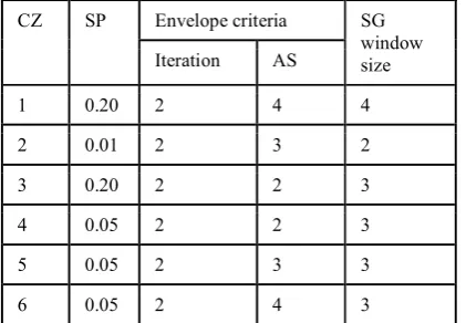
study area. TIMESAT software has options to fit a smooth continuous curve to time series of NDVI data using Savitzky-Golay (SG), Asymmetrical Gaussion (AG), or Double logistic (DL) functions, and an adaptive upper envelope to account for negatively biased noise such as cloud (Jonsson & Eklundh. 2002, 2004). Indian agriculture differs greatly in terms of its time of sowing, cropping pattern, cropping intensity etc. Thus a single equation to fit NDVI temporal curve may not hold good across the area. To resolve this issue, Indian region was divided into different calibration zones, based on NDVI time series principal component analysis (TS-PCA), to select smoothening techniques and its associated parameters settings (Heumann et al., 2007). Potential kharif agricultural mask is prepared from multi-year land use land cover map using AWiFS data. To cope up with the difference in spatial resolution between GIMMS NDVI (8 km) and AWiFS (60m), majority rule approach was adopted to aggregate the potential kharif agricultural area mask to coarse GIMMS NDVI. The mask is applied to subset kharif agricultural area over India and processed further to extract information of crop phenology. NDVI images of the first fortnight of each month of the year 1984, 1995 and 2006 (probable normal year from each decade) were selected to perform TS-PCA. First three TS-PCA components explained 96.8% of variance. Six zones for calibration were identified iteratively by isodata clustering technique using these first three TS-PCA components. These six calibration zones have six distinct temporal responses of NDVI (figure 1). Savitzsky-Golay filter (Chen et al., 2004) was used with different seasonality parameters, envelope adaptation strengths and window sizes to smoothen of temporal NDVI profile over the calibration zones (Table 1). Smoothened NDVI and original NDVI of total time series was compared with least square techniques and majority of the area showed R2 > 0.9. All the pixels were found to be significant (p = 0.05) under F-test.
CZ SP Envelope criteria SG
Table 1. Variable settings of parameters of Savitzky-Golay filter of TIMESAT over different calibration zones.(CZ: Calibration Zones, SP: Seasonality Parameters, AS: Adaptation Strength) 2.3 Computation of crop phenology matrices
There are several phenology matrices that can be extracted from time series NDVI data using TIMESAT software (Fig 2). The present study analyzed three important phenology matrices i.e. start of the growing season (SGS), seasonal NDVI amplitude (AMP), seasonal greenness or seasonally integrated NDVI (SiNDVI) during kharif season. In general, there are two
approaches for determining the SGS from the seasonal variation in NDVI. The first method uses a NDVI threshold to identify the beginning of photosynthetic activities in monsoon /kharif period. The second one identifies the period of large increase in NDVI as the beginning of growing season. A limitation associated with the threshold approach is that various land use types requires the use of different thresholds.
Since most of the agricultural area of India varied greatly in the soil & crop type, time of showing etc, determining the optimal threshold value for whole India would be difficult. Thus, the second approach was used in the present study. The SGS were estimated as the time point at which the value of the fitted function has first exceeds 20% of the distance between minimum and miximum at the rising limb. During calibration, it was found that estimation of SGS using values less than 20% had increased error due to noise effects. AMP is defined as the difference between the base and maximum NDVI values. SiNDVI is defined as the area under the vegetation curve during the growing season and above the mean of the base value.
2.4 Spatial trends of crop phenology matrices
Anomalies of the crop phenology matrices from its long term mean were calculated and trend of it were analyzed using nonparametric statistical approach. The Mann-Kendall test was employed to detect presence of trends of phenology matrices, while Sen’s method was used to compute the magnitude of the change. The advantages of this method over parametric statistics are that the missing values in time series data are allowed and the data do not require to conform any particular distribution. The Mann-Kendal test searches for a trend in a time series without specifying whether the trend is linear or nonlinear. Mann-Kendall method firstly calculates S statistic, which indicates the sum of the difference between the data points indicated in following equation.
(1)
Where, xi is observed value at time j, xk is observed value at time k, j is time after time k and n is the length of the data set. The sign of the value is defined as follows:
The value of S indicates the direction of trend. A negative (positive) value indicate falling (rising) trend. Mann- Kendall have documented that when n 8 , the test statistics S is approximately normally distributed with mean and variance as follows:
# (3)
$%& '( +,-.)*)*')*(
/ (4)
Where n indicates the number of data points, q indicates the number of tied groups (a tied group is a set of sample data having the same value) and t indicates the number p of data points in the pth group.
The statistical significance of S is checked using a test statistic (or Z score). The standardized Mann-Kendall statistics Z follows the standard normal distribution with zero mean and unit variance.
0
The Mann-Kendall method test the null hypothesis, H0 , is that data indicate no distinct trend against the alternative hypothesis Hi is that data indicate a trend. Two tailed test is used to decide whether or not the null hypothesis should be rejected in favour of hypothesis test. The null hypothesis, H0 is tested by the Z test statistic value. A decreasing trend is identified if Z is negative and an increasing trend is identified if the Z is positive. In the present study, H is rejected at p = 0.1 if the absolute value of Z is greater than Ztab , where Ztab is taken from the standard normal cumulative distribution tables.
Linear regression method is generally used to estimate the slope of possible linear trend in time series but for noisy (outliers or missing data) short time series data it may grossly miscalculate the magnitude of trend. Sen’s slope estimator is robust non-parametric trend operator and is highly immuned to gross data error (Sen., 1968). The break down bound of Sen’s estimator is approximately 29%. Thus the estimated trends have to have persisted for more than 29% of the length of the time series. In the present study, magnitude of the trend over time is estimated according to Sen et al., 1968. It is calculated by determining the possible slope between all possible data pairs and then finding the median value as under;
7 898:
(6)
Where, Qi is slope between data points, xi is data measure-ment at time j, xk is data measurement at time k and j > k.
2.5 Field significance test
For each grid cell, and separately for SGS, AMP and SiNDVI anomalies data, Mann-Kendall test (at p= 0.1) for the null hypothesis of no trend were performed. While analyzing phenology matrices during kharif season over a large region like India to identify trends, it is also important to ascertain the computed trend across that region using the field significant test (Livezey and Chen, 1983). Field significant test is performed over each meteorological subdivision (field or global). First the trend is computed at each individual grid level and the number of grid having trends (increasing/decreasing) are used as an input to the field significant test for checking the hypothesis that the respective meteorological subdivision has any trend (increasing/decreasing).
In terms of the probability theory, a collection of N independent significance tests (trend analysis of N grid points) is perfectly analogous to N tosses of a loaded coin. Instead of Heads or Tails,
with odds based on the coin load, the outcome for a 0.1 significance level test is passed (probability equal to 0.1) or test failed (probability equal to 0.9). This can be modeled with a binomial distribution as under;
;&< =
> ?> ?=> (7) Where M = 0, 1, 2, ...
The field significant test is considered to be passed if the number (M) of individual tests passing (out of N tests), with a significance level 0.1, exceeds a threshold number (M0). As an example, a meteorological subdivision having 40 grids is tested for trends using Mann-Kendal test at p=0.1. As per binomial distribution (equation 7), the probabilities are exactly 0.01478, 0.06569, 0.014233, 0.20032, 0.20588, 0.16471 and 0.10676 for 0, 1, 2, 3, 4, 5 and 6 passed tests out of 40 grids. Thus, the cumulative probabilities are 0.20627 for five or more passed test and 0.099517 for six or more. Therefore, if field significant test of a meteorological subdivision (having 40 grids) is performed, minimum six grids (threshold number, M0) must pass (significant at p = 0.1) to guarantee at least 90% (in this case 0.90048%) significance. Following this procedure, threshold number (M0) of grids having significant trend were computed for each meteorological subdivision at 90% level of significance. The meteorological subdivisions were declared to have significant trend (increasing/decreasing) if total grids with significant trend (increasing/decreasing) is equal or more than the threshold number (M0).
3 RESULTS AND DISCUSSIONS
Grid wise analysis of trends of kharif SGS, AMP and SiNDVI over different meteorological subdivisions are shown in Table 2. The numbers of grids having trend (positive/negative) or no trend are presented as N in Table 2. Number of grids showing significant trend (at p= 0.1) both in case of positive and negative are shown in brackets. Average magnitudes of trend (sen’s method) separate for positive and negative categories over each meteorological subdivision are presented as slope in Table 2. Meteorological subdivisions passed “field significance test” at p=0.1 are shown as bold.
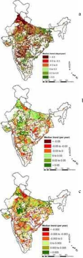
Spatial pattern of median trend of kharif SGS using GIMMS NDVI data for the period of 1982-2006 is presented in Fig. 3a. Strong negative trend (> -0.3 days/year) of SGS i.e. advancement of kharif season is observed over most of the part of north, central and western India. Positive trend of SGS i.e. delay in kharif season (>0.3 days/year) is found in eastern and southern part of India. Field significant test (at p=0.1) over the meteorological subdivisions revealed significant negative trend over Punjab 0.77 days/year), Haryana 0.57days/year), Marathwada (-0.75days/year), Vidarbha (-0.61 days/year) and Madhya Maharashtra (-0.1 days/year). Whereas, significant positive trend is observed over Rayalaseema (0.94 days/year), Coastal Andhra Pradesh (1.24 days/year), Bihar (1.1 days/year), Gangetic west Bengal (0.94 days/tear) and Sub-Himalayan West Bengal (1.6 days/year).
India. Southern and western part showed negative trend of SiNDVI. Statistically significant positive trend of SiNDVI (0.02 to 0.05 year-1) was found over Punjab, Haryana, West & East Uttar Pradesh, West & East Rajasthan, West Madhya Pradesh, Sourastra & kutch, Rayalaseema, Marathwada, Vidarbha, Bihar and Sub-Himalayan West Bengal. Statistically significant negative trend of SiNDVI (-0.02 to -0.04 year-1) was found over Tamilnadu, South Interior Karnataka, Coastal Andhra Pradesh, Madhya Maharashtra, Chhattisgarh, Gujarat and Gangetic West Bengal. East Madhya Pradesh passed field significant test both for positive and negative categories. Northern part of East Madhya Pradesh showed significant positive trend where as southern part shown significant negative trend of SiNDVI.
Spatial pattern of median trend of kharif season NDVI amplitude or crop vigour (fig.3c) showed positive trend over north, east, central regions of India, where as southern part shown negative trend. Statistically significant positive trend of AMP (0.002 to 0.007 year-1) is observed over Punjab, Haryana, West & East Rajasthan, East Uttar Pradesh, Bihar, Sub-Himalayan West Bengal, West Madhya Pradesh, Sourastra & Kutch, North Interior Karnataka, Rayalaseema. On the other hand, significant negative trend of AMP (-0.002 to -0.003 year-1) is found over Tamilnadu, South Interior Karnataka, Coastal Andhra Pradesh, Marathwada, Madhya Maharastra, Orissa, Gujarat and Jharkhand. Field significant test was found to be passed both for negative and positive trend in case of Telangana, Vidarbha, Chhattisgarh, Gangetic West Bengal, East Madhya Pradesh, West Uttar Pradesh. Parts of these meteorological subdivisions showed both significant positive and negative trend of kharif seasonal NDVI amplitude.
Figure 1. Study area with different calibration zones. Meteorological subdivisions under the present study: Punjab(1), Haryana Chandigarh Delhi (2), West Uttar Pradesh (3), East Uttar Pradesh (4), West Rajasthan (5), East Rajasthan (6), West Madhya Pradesh (7), East Madhya Pradesh (8), Gujarat region Daman DNH (9), Sourastra Kutch Diu (10), Chhattisgarh (11), Jharkhand (12), Bihar (13), Sub-Himalayana West Bengal (14), Gangetic West Bengal (15), Orissa (16), Telangana (17), Coastal Andhra Pradesh (18), Rayalaseema (19), Madhya Maharashtra (20), Marathwada (21), Vidarbha (22), North Interior Karnataka (23), South Interior Karnataka (24), Tamil Nadu and Pondicherry (25).
Figure 2. Crop phenology matrices estimated using the software TIMASAT- start of growing season (SGS), end of growing season (EGS), length of growing season (LGS), date of maximum NDVI (dMAX), Seasonal NDVI amplitude (AMP), and seasonally integrated NDVI (SiNDVI). (from Jonsson & Eklundh, 2002)
Fig. 3 Spatial pattern of median trend (Sen’s slope) of (a) SGS, (b), SiNDVI (c) AMP during kharif season using GIMMS NDVI data for the period of 1982-2006.
a
c b
.Table 2. Grid wise trend of Start of growing season (SGS), seasonal NDVI amplitude (AMP) and Seasonal integrated NDVI (SiNDVI) during kharif season using GIMMS NDVI data for the period of 1982-2006
N = Number of grids having positive/negative trend, Number of grids showing significant trend (p = 0.1) are presented in brackets, Average magnitude of trend (positive or negative) estimated by Sen’s method are presented as slope (days/year for SGS; year-1 for AMP and SiNDVI), Meteorological subdivisions passed “field significant test” at p=0.1
are marked as bold.
4 CONCLUSIONS
Present study found out two kinds of greening trends over Indian region during kharif season. Increasing SiNDVI along with increase in AMP was observed over Punjab, Haryana, West & East Uttar Pradesh, West & East Rajasthan, West & East Madhya Pradesh, Bihar, Sub-Himalayan West Bengal, Sourashtra & Kutch and Rayalaseema. Whereas, increasing SiNDVI along with decreasing of AMP was found over Marathawada, Vidarbha implying increase of the length of the growing. Significant browning trends during kharif season were observed in most of the south and eastern part of India covering Tamilnadu, South Interior Karnataka, Coastal Andhra Pradesh, Madhya Maharashtra, Gujarat region, Chhattisgarh, Jharkhand and Gangetic West Bengal. Shifts in the crop phenology matrices are a composite effect of climate and anthropogenic interventions such as introduction of new crop /crop varieties or management practices or irrigation facilities etc. Further research work is required to analyze the functional relationship between different causative factors (anthropogenic and climatic) and shifts in crop phenology matrices.
REFERENCES
Chen, J., Jönsson, P., Tamura, M., Gu, Z. H., Matsushita, B., Eklundh, L., 2004. A simple method for reconstructing a high-quality NDVI time-series data set based on the Savitzky–Golay filter. Remote Sensing of Environment, 91(4), pp. 332−344. Cleland, E. E., Chuine, I., Menzel, A., 2007. Shifting plant phenology in response to global change. Trends in Ecology and Evolution, 22, pp. 375-365.
Fisher, J. I., Richarson, A. D., Mustard, J. F., 2007. Phenology model from surface meteorology does not capture satellite based greenup estimation. Global Change Biology, 13, pp. 707-721. Fontana, F., Rixen, C., Jonas, T., Aberegg, G., Wunderle, S., 2008. Alpine grassland phenology as seen in AVHRR, Vegetation, and MODIS NDVI time series- a comparison with in-situ measurement. Sensor, 8, pp. 2833-2853.
Heumann, B.W., Seaquist, J.W., Eklundh, L., Jonsson, J., 2007. AVHRR derived phenological change in the Sahel and Soudan, Africa, 1982-2005. Remote Sensing of Environment, 108, pp. 385-392.
Jönsson, P., Eklundh, L., 2002. Seasonality extraction by function fitting to time-series of satellite sensor data. IEEE Transactions on Geoscience and Remote Sensing, 40, pp. 1824−1832.
Jönsson, P., Eklundh, L., 2004. TIMESAT—A program for analyzing timeseries of satellite sensor data. Computers & Geosciences, 30, pp. 833−845.
Kariyeva, J., van Leeuwen, W. J. D., 2011. Environmental drivers of NDVI based vegetation phenology in Central Asia. Remote Sensing, 3, pp. 203-246.
Livezey, R. E., Chen, W. Y., 1983. Statistical field significance and its determination by Monte Carlo technique. Monthly Weather Review, 111, pp. 46-59.
Melendez, P. I., Pedreno, J. N., Koch, M., Gomez, I., Hernandez, E., 2010. Land-cover phonologies and their relation to climatic variables in an anthropogenically impacted mediterranean. Remote Sensing, 2, pp. 697-716.
Menzel, A., Estrella, N., Fabian, P., 2001. Spatial and temporal variability of the phenological seasons in Germany from 1951 to 1996. Global Change Biology, 7, pp. 657-666.
Penuelas, J., Fiella, I., 2001. Response to a warming world. Science, 294, pp. 793-794.
Schaber, J., Badeck, F. W., 2003. Physiology based phenology models for forest tree species in Germany. International Journal of Biometeorology, 47, pp. 193-201.
Sen, P. K., 1968. Estimation of regression coefficients based on Kendall’s tau. Journal of American Statistical Association, 63, pp. 1379-1389.
Soudani, K., Maire, G., Dufrene, E., 2008. Evaluation of the onset of greening-up in temperate deciduous broadleaf forests derived from Moderate Resolution Imaging Spectroradiometer (MODIS) data. Remote Sensing of Environment, 112, pp. 2643-2655. Stockli, R., Vidale, P. L., 2004. European plant phenology and climate as seen in a 20 year AVHRR land surface parameters dataset. International Journal of Remote Sensing, 25(17), pp. 3303-3330.
Tao, F., Yokozawa, M., Xu, Y., Hayashi, Y., Zhang, Z., 2006. Climate change and trend in phenology and yield of field crops in China, 1981-2000. Agriculture and Forest Meteorology, 227 , pp. 369-375.
Tucker, C. J., Pinzon, J. E., Brown, M. E., Slayback, D. A., Pak, E. W., Mahoney, R., 2005. An extended AVHRR 8-km NDVI dataset compatible with MODIS and SPOT vegetation NDVI data. International Journal of Remote Sensing, 26(20), pp. 4485−4498.
Van Leeuwen, W. J. D., Davison, J. E., Casady, G. M., Marsh, S. E., 2010. Phenology characterization of desert sky island vegetation communities with remotely sensed and climate time series data. Remote Sensing, 2, pp. 388-415.
Zhou, L.M., Tucker, C.J., Kaufmann, R.K., Slayback, D., Shabanov, N.V., Myneni, R., 2001. Variation in northern vegetation activity inferred fron satellite data of vegetation index during 1981 to 1999. Journal of Geophysical Research-Atmosphere, 106, pp. 20069-20083.
ACKNOWLEDGEMENTS:
We would like to thank Dr. V. K. Dadhwal, Director NRSC, ISRO for his constructive suggestions. Tucker et al., 2004 is duly acknowledged for providing GIMMS NDVI data set. The TIMESAT software is available online in http://www.nateko.lu.se/personal/Lags.Eklundh/TIMESAT/times at.