www.elsevier.comrlocateratmos
Statistical characteristics of interdecadal
fluctuations in the Southern Oscillation and the
surface temperature of the equatorial Pacific
Omar Abel Lucero
), Norma C. Rodrıguez
´
( )Instituto Nacional del Agua y del Ambiente CRS , National UniÕersity of Cordoba, Pasaje Curupaity 2460,´
5009 CordoÕa, Argentina
Received 21 July 1998; accepted 10 January 2000
Abstract
Decadal and interdecadal fluctuations in the Southern Oscillation index, SOI, and in the SSTI
ŽWright’s sea surface temperature index of the equatorial Pacific are the focus of this research.. Ž .
The SSTI is defined by the average anomaly of sea surface temperature SST in regions of the eastern and central equatorial Pacific. Analyses were carried out using the integral wavelet transform. Full understanding of the climate variability that takes place within a century or smaller timescale requires knowing the characteristics of these fluctuations. The following findings are
Ž .
documented in this paper. 1 The interfluctuation span in decadal and bidecadal components of SOI and SSTI are normally distributed; standard deviation values cast doubts on the potential of
Ž .
statistical models for long-term — 10 to 20 years ahead — forecasting. 2 There is a large
Ž .
correlation between positive negative extreme of SOI fluctuations and associated negative
Žpositive extreme of SSTI fluctuations at decadal, bidecadal, and interdecadal timescales. 3 In. Ž .
mid-1930s, a change in the relative phase between decadal fluctuations of SOI and SSTI occurred.
Ž .4 Early 1960s pulsations at decadal and total interdecadal timescales of SOI and SSTI started to
Ž .
amplify. 5 Summer bidecadal components of SOI and SSTI started to amplify at about
Ž .
mid-1930s, whereas winter bidecadal components do not show amplification. 6 Signals in the band of wavelet timescale smaller than 10 year — encompassing ENSO signals — do not show
Ž . Ž .
indication of climate variability throughout the period of study 1896–1985 . 7 The controlling process on the variability of the decadal components of winter SOI and winter SSTI during that
Ž
period is a joint amplitude modulation for brevity, denominated amplitude modulation of decadal
)Corresponding author. Tel.:q54-0351-4883317.
Ž .
E-mail address: [email protected] O.A. Lucero .
0169-8095r00r$ - see front matterq2000 Elsevier Science B.V. All rights reserved. Ž .
observed in this century in the values of these two indexes. The modulation of the decadal component of SSTI is clearly seen in summer and winter averages.q2000 Elsevier Science B.V.
All rights reserved.
Keywords: Interdecadal fluctuations; Southern Oscillation; Equatorial Pacific
1. Introduction
Decadal and interdecadal climate variability affects water resources and agricultural production in many regions of the world. Often, this climate variability is wrought in the
Ž .
form of quasi-periodic fluctuations in atmospheric variables. A few examples are 1 a rainfall climate change of multidecadal extent starting in mid-1930s in the southern
Ž .
mid-latitudes Lucero and Rodrıguez, 1999 , formed by 12- and 20-yearr period
´
Ž .
amplifying fluctuations. 2 Rainfall variations spanning cycles of 12 and 20 years in
Ž .
central United States Hu et al., 1998 ; and interdecadal fluctuations in precipitation in
Ž .
US Pacific coast Chen et al., 1996 .
Ž .
Decadal and interdecadal fluctuations in the Southern Oscillation SO and in the sea
Ž .
surface temperature SST of the equatorial Pacific are suspected to contribute to the generation in several parts of the world of rainfall fluctuations with the same timescales. Observational verification of this influence requires first to know in more detail some of the statistical characteristics of the SO and the SST in the equatorial Pacific.
We report on some of the characteristics of decadal and interdecadal fluctuations in
Ž .
the equatorial Pacific SST and in the Southern Oscillation index SOI . The approach is statistical and observational. These fluctuations are embedded in the interdecadal variability originating in the Tropics, which is one of the four major types of
atmo-Ž .
spheric decadal and interdecadal variability Latif, 1998 .
The data description and methodology is described in Section 2. The rationale and the
Ž .
blueprint of the paper are the following. 1 The probability distributions of the time
Ž
between consecutive fluctuations in SOI and SSTI sea surface temperature index of
.
Wright, 1989 at decadal and interdecadal timescales are unknown. This topic is
Ž .
analyzed in Sections 3.1 and 3.2. 2 A search in the literature shows no observational quantitative evidence on the relationship between amplitudes of decadal and interdecadal components of the SOI and the SSTI. The SOI is a measure of the average gradient of surface pressure across the tropical Pacific, thus it is also a measure of the average surface wind stress on that region. Therefore, a relationship between amplitudes of decadal and interdecadal components of SOI and of SSTI is tantamount to a relationship
Ž
between wind stress and sea surface temperature on the equatorial Pacific Clarke and
.
Lebedev, 1996 . That relationship between fluctuations of SOI and SSTI is described in
Ž .
Section 3.4. 3 A topic insufficiently studied is the relative phase between simultaneous fluctuations of SOI and SSTI at decadal and interdecadal timescales. Changes in the
Ž .
Long-term modulation of decadal and interdecadal fluctuations in annual rainfall amount has been found by other authors. For finding the explanation of that modulation, it is of interest to know if there is a joint amplitude modulation of decadal and interdecadal fluctuations of SOI and of SSTI. Although indication of long-term modulation of time series of SST is found in the literature, it has not been documented a joint amplitude modulation of the decadal and interdecadal components of the SOI and the SST in the equatorial Pacific during this century. The existence and characteristics of a joint amplitude modulation is described in Section 3.6. Finally, Section 4 contains a discus-sion of results, and Section 5 contains a summary of findings.
2. Data and methodology
2.1. Data
Ž .
A monthly SSTI was obtained from Wright 1989 . This index is defined as the
w x w
monthly mean of SST anomaly over the region 6–28N, 170–908W ; 28N–68S, 180–
x w x
908W , and 6–108S, 150–1108W ; this region is in the central and eastern equatorial
Pacific. SSTI can take on positive as well as negative values. The time series of monthly values of SST index covers the 104-year interval 1882–1985. Values of SSTI are given in degree-Celsius.
Ž .
The operational SOI of the Climate Prediction Center CPC of NOAA is used in this research. SOI data covers the 101-year interval 1896–1996. The SOI is defined as:
SOIs
Ž
TsyDs.
rM ,swhere T is the standardized monthly mean of sea level pressure in Tahiti; standardizeds
Ž
Darwin, D , is similarly defined. A variable is standardized if its mean value is zeros .
and its standard deviation is 1 . M is given by:s
1 2
Mss
(
ÝŽ
TsyDs.
, where Nstotal number of summed months.N
Two sets of yearly data were constructed from the monthly SOI time series and from
Ž
the monthly SSTI time series. One set is the average from November to April ‘summer
.
season’ . Summer and winter months correspond to the Southern Hemisphere. The other
Ž .
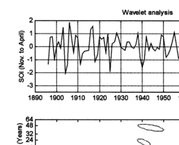
set is the average from May to October ‘winter season’ . The time series of summer SOI is shown in the upper panel of Fig. 1. The time series of summer SSTI is shown in Fig. 6. Hereafter, SOI and SSTI refer only to seasonal averages.
2.2. WaÕelet analysis
Time-varying components at different frequencies, of both SSTI and SOI, are individualized using the Morlet continuous wavelet transform. Wavelet analysis is increasingly being used in atmospheric sciences to analyze time series of several types
Ž .
Fig. 1. Top panel: Observed summer SOI. Bottom panel: Contributions to summer SOI, at indicated years
Ž . Ž .
from indicated wavelet period. Dotted solid contours indicate negative positive contributions.
Ž .
Following Torrence and Compo 1998 , let xn be a time series of a variable X,
where ns0 . . . Ny1; measurements are equally spaced at time interval dt equal to 1
year. In this research, the variable X is equal to the 6-month average of SOI or SSTI. After wavelet decomposition of the time series made up of values x , the reconstructionn
is given by:
J R W s
Ž .
n jxnsA
Ý
s1r2 j js0w Ž .x
where A is a constant, R W sn j is the real component of the complex wavelet
transform, and s is the wavelet scale, J is the largest scale. To avoid unnecessaryj
Ž .
repetition, readers are referred to Torrence and Compo 1998 for details of the Morlet continuous wavelet transform.
Results of wavelet analysis are presented as a time series for contributions xn , j for each scale j as function of time n. For example, in Fig. 1, the upper panel shows the original time series of summer SOI. The bottom panel of this figure shows the time
4 Ž .
series xn , j, for all scales j js2, . . . ,64 . Ordinate unit is the wavelet period in years
Ž .
corresponding to each scale. In this figure, negative positive contours indicate negative
Žpositive contributions to the value of the SOI. The sign of the contribution of each.
Ž .
wavelet period indicates whether contribution increases positive sign or decreases
In this paper, the term wavelet period is used instead of wavelet scale. Wavelet scale is converted in such a way that if the analyzed wave is a periodic cosine or sine function, the wavelet spectrum will be equal to Fourier spectrum. In the case of the Morlet wavelet, the conversion factor is ls1.03 s, where s is the scale and l is the
equivalent period in Fourier representation. For the Morlet wavelet, the wavelet scale is
Ž .
almost equal to that Fourier period; see Torrence and Compo 1998 and Meyers et al.
Ž1993 for more details..
2.3. Partial contribution from bands of waÕelet period
A convenient identification and description of the intensity of fluctuations is achieved
Ž .
summing the contributions from wavelets with scaling wavelet period within a given
Ž . Ž .
interval Lucero and Rodrıguez, 1999 . The contribution from an interval a band of
´
Ž .
wavelet period is called component of the SOI or of the SSTI in that band. Fig. 2 shows five components. Selection of intervals of wavelet period was carried out based
Ž
on results of other authors on period of climatic fluctuations Trenberth and Hurrell,
.
1994; Knutson and Manabe, 1997, among others .
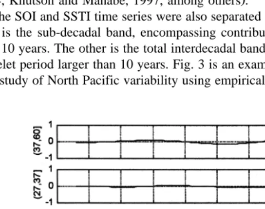
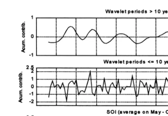
The SOI and SSTI time series were also separated out into two bands of contribution. One is the sub-decadal band, encompassing contributions from wavelet period smaller than 10 years. The other is the total interdecadal band, encompassing contributions from wavelet period larger than 10 years. Fig. 3 is an example of this partitioning of the SOI. In a study of North Pacific variability using empirical orthogonal functions, Zhang et al.
Fig. 3. Partial contribution to winter SOI from bands of wavelet periods as indicated on top of upper and middle panel. Bottom panel is observed winter SOI.
Ž1997 also partitioned the global SST field into two components: ENSO-like timescale,.
and total interdecadal timescale.
2.4. Computation of lag
In this research, the interest is in the lag between extremes of opposite signs of SOI and SSTI because out-of-phase SOI and SSTI signals are commonly assumed to interact constructively. This type of lag is denominated Lag-BFOS for ‘lag between fluctuations
Ž .
of opposite sign’, and it is identified by the lag of the relative minimum negative value
Ž .
of the cross-correlation function closest to lag zero see Fig. 14 . Positive lag-BFOS indicates that the SOI signal leads the SSTI signal. Results are expressed in units of year. A lag-BFOS equal to zero year is equivalent to a conventional lag equal to 1808.
2.5. Definitions
For ease of reference, definitions of some terms used in this paper are given in this
Ž
section. The band including contributions from wavelet period within the interval 10 to
x Ž .
17 years is denoted decadal band. The band 17 to 27 years is the bidecadal band. The band including contributions from wavelet periods larger than 10 years is denoted
Ž .
the total interdecadal band. An expression like decadal component of SOI or SSTI
Ž x
has the meaning of ‘partial contribution from the band 10 to 17 years to the
Ž .
reconstruction of SOI or SSTI ’. A fluctuation, or a pulsation, refers to a
non-sta-Ž
tionary feature bounded in time by two consecutive extremes of the same type For
.
are not periodic, fluctuations generally do not repeat at equal interval of time. The span between two specific consecutive maximum, or minimum, of SOI or SSTI is used to
Ž .
identify the corresponding interfluctuation period or interfluctuation span . The words
signal or component refer to the contribution from a band along the length of data
record, or along another specified period.
3. Results
3.1. Fluctuations in the atmospheric mass oÕer the tropical pacific
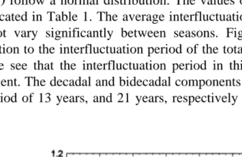
Fig. 2 shows five contributing bands to summer SOI from indicated wavelet periods
Žthe figure for winter SOI is not shown . The sub-decadal component is shown in the.
second panel from bottom. The remaining upper panels show the decadal and the other interdecadal components.
Ž .
The main features shown in Fig. 2 are: 1 an amplification of the bidecadal
Ž .
component starting in mid-1930s, 2 an amplification of the decadal component starting
Ž .
early 1960s. 3 A weak tridecadal component. We analyze next the total interdecadal component of SOI; the other components are analyzed in following sections.
The total interdecadal component of winter SOI is singled out in the upper panel of
Ž .
Fig. 3 Summer components of SOI is similar, as seen in Fig. 4 . Main features are as follows.
Ž .1 There is an amplitude modulation of the interdecadal component of the SOI. Apparently, a cycle of the amplitude modulation goes from around 1905 to mid-1970s.
Ž .
This suggests a 70-year span amplitude modulation for this realization sample of 100-year extent.
Ž
Fig. 4. Contributions to winter SOI and to summer SOI, from total interdecadal band wavelet period)10
.
Decadal Winter 13.1 1.8
Summer 12.8 1.6
Bidecadal Winter 22 2.7
Summer 19.2 6.0
Total interdecadal Winter 15.6 4.7
Summer 12.8 2.3
Ž .2 In 1982, year of a strong ENSO, the winter SOI reaches a large negative value Žsee bottom panel of Fig. 3 that was attained with the strong negative contribution from.
Ž .
the interdecadal band Figs. 3 and 4 . This results supports suggestions made by
Ž . Ž .
Brassington 1977 and Zhang et al. 1998 , based on indirect evidence obtained using Fourier and principal component analyses respectively, on the existence of a construc-tive interaction between decadal and sub-decadal signals of the SOI.
A Kolmogorov–Smirnov test of goodness-of-fit indicates that inter-fluctuation
peri-Ž
ods in the decadal, bidecadal and total interdecadal components of SOI winter and
.
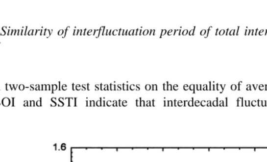
summer follow a normal distribution. The values of the parameters of the distributions are indicated in Table 1. The average interfluctuation period for these three components does not vary significantly between seasons. Fig. 5 shows the fitting of a normal distribution to the interfluctuation period of the total interdecadal component of summer SOI; we see that the interfluctuation period in this case is dominated by the decadal component. The decadal and bidecadal components of SOI have an average
interfluctua-Ž .
tion period of 13 years, and 21 years, respectively after averaging on both seasons .
Fig. 6. Partial contributions to summer SSTI from bands of wavelet period as indicated in the y-axis. Year corresponds to November. The vertical scale is stretched for period greater than 10 years, to better depict signal features.
3.2. Fluctuations of the sea surface temperature in the equatorial Pacific
Fig. 6 shows partial contributions to the reconstruction of summer SSTI. Among components with wavelet period )10-year, partial contributions from the decadal band are the largest. The magnitude of the bidecadal component is second in importance. Partial contributions to SSTI from bands encompassing wavelet period larger than 27 year are small.
Seasonal differences in interdecadal components of winter and summer SSTI, Fig. 7, are not significant. There is an important maximum of SSTI centered in 1901. In
Decadal Winter 13.8 1.2
Summer 11.6 2.9
Bidecadal Winter 20.5 0.6
Summer 20.2 0.5
Total interdecadal Winter 13.3 1.6
Summer 11.4 2.6
mid-1940s, the quasi-regular pattern of pulsation changes into an almost linear
ascend-Ž .
ing warning trend. A new change occurs in early-1960s. Thereafter, the signal
amplifies. In another section, these features are related to changes in SOI.
Kolmogorov–Smirnov goodness-of-fit tests indicate that interfluctuation period for decadal, bidecadal and interdecadal components of SSTI follows a normal distribution; average values and standard errors are shown in Table 2. Fig. 8 shows the fitting of a normal distribution to the interfluctuation periods observed in the interdecadal band of summer SSTI. Standard error values cast doubts on the potential of statistical models for long-term — 10- to 20-year ahead — forecasting.
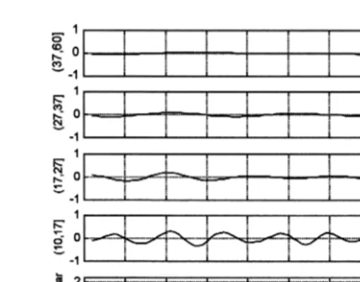
3.3. Similarity of interfluctuation period of total interdecadal component in SOI and in SSTI
A two-sample test statistics on the equality of average interdecadal oscillation period of SOI and SSTI indicate that interdecadal fluctuations in SSTI and SOI have a
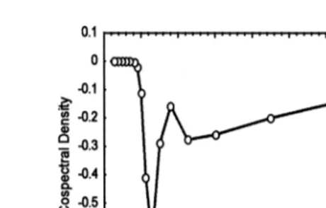
Fig. 9. Co-spectral density between total interdecadal component in summer SOI and summer SSTI. The 13-year wave period produces the largest contribution to cross-correlation between signals.
Ž
dominant cadence with an average period equal to 13 years. Co-spectrum analysis Fig.
.
9 also indicates that SSTI and SOI signals are out of phase, with a negative peak value at 13-year period. Negative sign of co-spectrum peak indicates that these components of SOI and SSTI are out of phase. The co-spectrum measures the contribution of oscilla-tions of different frequencies to the total cross covariance at lag zero between the time
Ž .
series of SOI and SSTI Panofsky and Brier, 1968 .
3.4. Statistical relationship between amplitudes of fluctuations of SOI and SSTI
A linear regression between the amplitudes of associated extremes of opposite sign of SOI and SSTI were carried out. ‘Associated extremes of opposite sign’ means that each
Ž . Ž .
positive negative extreme of SOI is related to the closest negative positive extreme of SSTI. Table 3 shows the results for three components. Amplitudes are negatively
Table 3
Liner regression between the value of an extreme in SOI and the closest extreme of opposite sign in SSTI, at indicated components
Null hypothesis is ‘‘slope of linear regression is zero’’, and it is rejected if p-level is smaller than 0.05. r is the value of the linear correlation coefficient. Test statistics is Student’s t.
Component Season Linear regression p-level r
Žslope.
Ž .
Total interdecadal Winter SSTI s0.049–0.70 SOI q´0, 0.157 0.0006 y0.84
ID ID
Ž .
Summer SSTIIDs0.048–0.54 SOIIDq´0, 0.226 0.011 y0.68
Ž .
Decadal Winter SSTIDe cs0.006–0.639 SOIDecq´ 0, 0.070 0.00001 y0.91
Ž .
Summer SSTIDe cs0.007–0.722 SOIDecq´ 0, 0.143 0.001 y0.79
Ž .
Bidecadal Winter SSTIBidcs0.004–0.894 SOIBidcq´ 0, 0.061 0.001 y0.92
Ž .
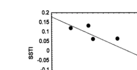
Fig. 10. Regression between peak value of summer SSTI, on value of associated extreme of opposite sign of summer SOI, in the bidecadal band. Correlation coefficient isy0.91.
correlated at a significance level of 5%. Fig. 10 is a graphical example of results for the summer bidecadal components of SOI and SSTI.
After a sudden decrease of amplitude, the bidecadal component of SSTI is amplifying
Ž .
since 1915 see Fig. 11 . Amplitudes of bidecadal SOI are amplifying since start of record.
3.5. RelatiÕe phase between components of SOI and SSTI
In this section, an analysis of the relative phase between components of SOI and
Ž
SSTI is carried out; results are expressed in terms of lag-BFOS see Section 2.4 for
.
definition of lag-BFOS . Bidecadal, interdecadal, and decadal components of SOI and
Ž .
SSTI see Figs. 11–13 show a change in relative phase around mid-1930s. The
lag-BFOS between components of SOI and SSTI was computed using cross-correlation
Ž .
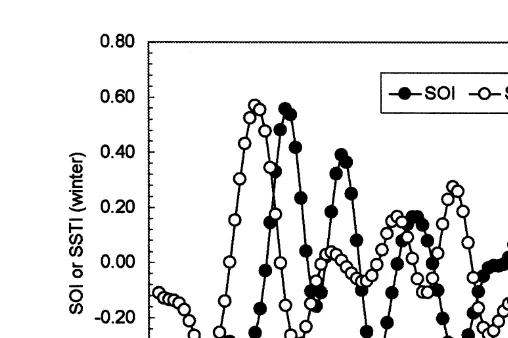
Fig. 12. Comparison of time series of total interdecadal component of winter SSTI and winter SOI.
analyses. Fig. 14 shows an example of cross-correlation analysis; this corresponds to the bidecadal winter components before 1935. Relative maximum of negative cross-correla-tion closest to zero lag is found at a lag of 2 years; positive lag corresponds to SOI leading SSTI. Table 4 shows the results of cross-correlation analyses. Before mid-1930s, the SOI component was leading the SSTI component at those three bands. After mid-1930s, the decadal and interdecadal components of SOI and SSTI are locked
Ž .
completely out of phase relative phase equal to 1808, or 0-year lag-BFOS8; while the
bidecadal component of SSTI leads the SOI component.
Ž .
In the tridecadal band figure not shown , the SSTI leads SOI throughout the period under study.
Fig. 14. Cross-correlation function between bidecadal winter SOI and bidecadal winter SSTI. Vertical axis is
Ž .
the lag year , horizontal axis is the cross-correlation value. Set of time series values before 1935. Positive lags
Ž
correspond to SOI leading SSTI. Relative maximum of negative cross-correlation closest to zero lag this is the
.
lag-BFOS is found at 2 years. Dashed lines enclose the 95% confidence interval.
3.6. Amplitude modulation of decadal SOI and SSTI
A conspicuous joint amplitude modulation controls the amplitude of the decadal
Ž .
components of winter SOI and winter SSTI Fig. 13 . In 1912, the decadal component of SOI reaches its deepest negative value. Thereafter, the negative extreme of the SOI
Ž . Ž
climbs to its highest value less negative in 1951. Then, it decreases again becomes
. Ž
more negative . Opposite evolution is observed in the relative maxima positive —
.
warmer — extremes of the decadal component of winter SSTI. The minimum
difference between an extreme of the decadal SOI and the corresponding extreme of opposite sign of the decadal SSTI is reached at 1957. After 1957, amplitudes amplify. This realization of the amplitude modulation covers about 70 years. Both summer and winter SSTI show the amplitude modulation in the decadal component. On the other hand, summer SOI do not show clearly the amplitude modulation of the decadal component.
Table 4
Ž .
Lag between fluctuations of opposite sign Lag-BFOS of SOI and SSTI Results were obtained using cross-correlation functions.
Component Season Lag-BFOS Conclusion Lag-BFOS Conclusions
Žyears before. Žyears after.
mid-1930s mid-1930s
Ž .
Decadal Winter 2 SOI leads 0 Out of phase 1808
Ž .
Summer 1 SOI leads 0 Out of phase 1808
Bidecadal Winter 2 SOI leads y2 SSTI leads
Summer 6 SOI leads y1 SSTI leads
Ž .
Total interdecadal Winter 3 SOI leads 0 Out of phase 1808
Ž .
4. Discussion
Several highly elaborated conjectures have been advanced on the physical processes that would produce decadal and interdecadal fluctuations in the SST in the equatorial Pacific. Although these conjectures were constructed from analyses of numerical simulations or simplified models of uncoupled and coupled ocean–atmosphere pro-cesses, it has yet to be presented empirical evidence supporting these conjectures. Findings in this research describe some properties of decadal and interdecadal fluctua-tions in equatorial SST and the SOI that ocean–atmosphere models would have to reproduce in support of those conjectures. In this section, we indicate some implications of these findings.
The regularity of the interfluctuation time of decadal and bidecadal components of SOI and SSTI suggests that some kind of wave mechanism could be the time regulator of the fluctuations. Results from some modeling studies indicate that fluctuations with a
Ž
decadal timescale or longer can be generated in the tropical Pacific Garreaud and
.
Battisti, 1999, Munnich et al., 1998, Zhang et al., 1998, and references therein . In this
¨
Ž .
research, peak values of positive negative SOI are unrelated to interfluctuation period. This latter result suggests that advection processes produced by wind stress may not be controlling the generation of decadal and bidecadal fluctuations.
Peaks of SOI fluctuations and associated peaks of opposite sign of SSTI fluctuations at decadal, bidecadal, and interdecal timescales are strongly and negatively correlated. This results support the prevalent postulate that at these long timescales a major control of anomalies of SST is the heat flux modulated by the wind speed anomalies. The SOI represents the average surface pressure gradient over the tropical Pacific, and thus it is also an index of surface wind speed. Immediate response of anomalies of SST to anomalies of wind speed would be expected. However, only after mid-1930s, decadal and bidecadal components of SOI and SSTI are completely out of phase. Before
Ž .
mid-1930s, fluctuations in SOI leads to fluctuation of opposite sign of SSTI at decadal and bidecadal timescale. This difference in relative phase before and after mid-1930s suggests that the relative importance of processes involved in the generation of decadal and bidecadal components of SOI and SSTI might have changed around that time.
Evidence was found on the occurrence of a joint amplitude modulation of the decadal component of the SOI and SSTI taking place along a period of about 70-year and attaining its minimum about 1957. After that time, decadal components are amplifying. These amplifying components contributed to the exceptional negative values of the SOI and to the high equatorial SST in early 1980s. This joint amplitude modulation of the decadal components of SOI and SSTI explains the large variations of those indexes since the start of the century. The question arises whether the change in relative phase in mid-1930s in the decadal and bidecadal components of SSTI and SOI produced changes in some surface atmospheric variables. Preliminary results from ongoing research indicate an affirmative answer. Contemporary to the above-described change of relative phase in mid-1930s, in central Argentina started a strong positive trend in annual rainfall
Ž .
amount Lucero and Rodrıguez, 1999 . This positive trend, which increased in early
´
research.
A century of data is not enough to determine if AMDecSO and the change of relative phase between decadal SOI and decadal SSTI are intrinsic to decadal processes in this atmospheric–oceanic system, or they are phenomena occurring only in this century. However, in the latter case, the question would arise about its possible link to global climate change. AMDecSO changes into a new type of oceanic–atmospheric coherent interaction at mid-1930s. The setting of an out-of-phase locking between decadal SOI and associated decadal SSTI component is not simultaneous to the start of amplification of decadal components. The change in relative phase occurs in mid-1930s, while amplitudes of SOI and SSTI signals keeps decreasing until about late 1950s. Early 1960s starts the amplification of SOI and SSTI signals. The perspective of a constructive interaction of SSTI and SOI signals leading to amplification of oscillation, in a new resilient decadal mode of oceanic–atmospheric interaction, is of concern.
5. Conclusion
Findings in this research are shown below.
Ž .1 The interdecadal components in seasonal SOI and seasonal SSTI have an
interfluctuation period normally distributed, with average value about 13 years and standard error of about 2 years. Cross-correlation analyses indicate that in the inter-decadal band before 1930s SOI leads the SSTI. After 1930s, there is no lag in associated fluctuations of opposite sign in SOI and SSTI.
Ž .2 Decadal and bidecadal fluctuations of SOI and SSTI also have an interfluctuation
Ž .
period normally distributed. Decadal fluctuations of SSTI SOI have an average
Ž .
interfluctuation time of 12.5 years 13 years . Bidecadal fluctuations of SOI and SSTI have an average interfluctuation time of about 20 years.
Ž .3 It was found that a statistically significant linear correlation between peak of SOI
Ž .
fluctuations and corresponding peak of opposite sign of SSTI fluctuations at decadal, bidecadal, and interdecal timescales.
Ž .4 A change in relative phase between decadal fluctuations of SSTI and SOI took place in mid-1930s. Before mid-1930s, component of SOI was leading SST component. After mid-1930s, decadal fluctuations of SSTI and fluctuations of opposite sign of SOI
Ž .
have a 0-year lag-BFOS they are completely out-of-phase ; there is also a change in the season with maximum amplitude of decadal and bidecadal SOI.
Ž .6 The relative phase between bidecadal component of SSTI and SOI changes about mid-1930s. Before mid-1930s, winter bidecadal fluctuations of SOI lead by 2 years the
Ž .
associated bidecadal fluctuations with opposite sign of winter SSTI; whereas after
Ž . Ž .
mid-1930s positive negative SSTI fluctuations lead to negative positive SOI fluctua-tions by 2 years. For summer, the same relafluctua-tionship holds, except that before mid-1930s SOI bidecadal fluctuations lead SSTI associated fluctuations of opposite sign by 6 years. After mid-1930s, summer SSTI bidecadal fluctuations are leading by 1 year to summer SOI bidecadal fluctuations. Summer bidecadal component of SSTI and SOI shows a rapid amplification starting mid-1930s.
Ž .7 Findings indicate that fluctuations in the tridecadal band are weak; this supports
Ž .
results from Timmermann et al. 1998 . Using an atmosphere GCM and an ocean model, these authors found that a coupled air–sea mode produces fluctuations with a period of about 35 years. However, their results indicate also that in the tropical regions, these fluctuations would be weak. The variability with 35-year period would be stronger at mid- and high-latitudes. These tridecadal fluctuations seem to be driven by the ocean because findings show that the SSTI component leads the SOI component of opposite sign. Tridecadal components are amplifying since mid-1930s
Ž .8 In early 1970s, the maximum in the subdecadal band of SOI is in-phase with the maximum in the decadal and bidecadal bands. Thereafter, fluctuations of total SOI amplify considerably. Contributions to total SOI from wavelet period larger than 17 years are negative during the 1980s. Early 1980s, the contributions from the decadal, bidecadal and tridecadal bands also become strongly negative, and contributed to the strongly negative values of total SOI attained during ENSO 1982r1983.
These results indicate that along this century there is a complex pattern of changes in decadal and bidecadal components to SOI and SSTI that are relevant for understanding climate variability.
Acknowledgements
Ž
This research was partially financed with a grant from CONICOR The Scientific
.
Research Council of Cordoba . The Centro de la Region Semiarida is a research center
´
´
´
Žof the National Institute of Water and Environment Instituto Nacional del Agua y del
.
Ambiente .
Ž
Drs. C. Torrence and G. Compo, at the University of Colorado Program in
.
Atmospheric and Oceanic Sciences , provided the software for wavelet decomposition of rainfall time series into a diagram ‘‘time-wavelet period’’. This wavelet software is available at http:rrpaos.colorado.edurresearchrwaveletsr.
References
Brassington, G.B., 1977. The model evolution of the Southern Oscillation. J. Clim. 10, 1021–1034.
Ž . Ž .
Latif, M., 1998. Dynamics of interdecadal variability in coupled ocean–atmosphere models. J. Clim. 11, 602–624.
Lucero, O., Rodrıguez, N., 1999. Relationship between interdecadal fluctuations in annual rainfall amount and´ annual rainfall trend in a southern midlatitudes region of Argentina. Atmos. Res, in press.
Meyers, S.D., Kelley, B.G., O’Brien, D.G., 1993. An introduction to wavelet analysis in oceanography and meteorology: with application to the dispersion of Yanai waves. Mon. Weather Rev. 121, 2858–2866. Munnich, M., Latif, M., Venzke, S., Maier-Reimer, E., 1998. Decadal oscillations in a simple coupled model.¨
J. Clim. 11, 3309.
Panofsky, H.A., Brier, G.W., 1968. In: Some Applications of Statistics to Meteorology. Pennsylvania State University Press, 224 pages.
Timmermann, A., Latif, M., Voss, R., Grotzner, A., 1998. Northern hemispheric interdecadal variability: a¨ coupled air–sea mode. J. Clim. 11, 1906–1931.
Trenberth, K., Hurrell, J.W., 1994. Decadal atmosphere–ocean variations in the Pacific. Climate Dynamics 9, 303–319.
Ž .
Torrence, C., Compo, G., 1998. A practical guide to wavelet analysis. Bull. Am. Meteorol. Soc. 79 1 , 61–78. Wright, P., 1989. Homogenized long-period southern oscillation indices. Int. J. Climatol. 9, 33–54. Zhang, Y., Wallace, J.M., Battisti, D.S., 1997. ENSO-like interdecadal variability: 1900–93. J. Clim. 10,
1004–1020.