EVALUATION OF SIFT AND SURF FOR VISION BASED LOCALIZATION
Xiaozhi Qu, Bahman Soheilian, Emmanuel Habets, Nicolas Paparoditis
Universite Paris-Est, IGN, SRIG, MATIS, 73 avenue de Paris, 94160 Saint Mande, France (firstname.lastname)@ign.fr
Commission III, WG III/4
KEY WORDS: Vision Based Localization, Local Bundle Adjustment, Feature Extraction, performance evaluation.
ABSTRACT:
Vision based localization is widely investigated for the autonomous navigation and robotics. One of the basic steps of vision based localization is the extraction of interest points in images that are captured by the embedded camera. In this paper, SIFT and SURF extractors were chosen to evaluate their performance in localization. Four street view image sequences captured by a mobile mapping system, were used for the evaluation and both SIFT and SURF were tested on different image scales. Besides, the impact of the interest point distribution was also studied. We evaluated the performances from for aspects: repeatability, precision, accuracy and runtime. The local bundle adjustment method was applied to refine the pose parameters and the 3D coordinates of tie points. According to the results of our experiments, SIFT was more reliable than SURF. Apart from this, both the accuracy and the efficiency of localization can be improved if the distribution of feature points are well constrained for SIFT.
1. INTRODUCTION
Localisation with Global Navigation Satellite Systems (GNSS) in dense urban areas suffers from masks of signals and multi-path errors and leads to significant errors. Dead reckoning methods using inertial navigation Systems (INS) were applied in order to reduce these errors by interpolating between GNSS interruptions. Vision based relative positioning methods such as visual odome-try can provide the same improvement at lower costs.
Nowadays, a variety of methods have been proposed for vision based localization (Davison, 2003; Nist´er et al., 2004; Mouragnon et al., 2006). The main steps of these methods can be summarized as: feature extraction, matching, pose estimation, and 3D struc-ture reconstruction. The reliable matching constitutes the basis of vision based localization (Valgren and Lilienthal, 2010). The local feature based methods have been proved to be an excellent choice for pose estimation. However, the factors such as illu-mination changes, perspective deformations and moving objects make the matching a difficult task and influence the accuracy of pose estimation.
Thus the algorithms used for local feature extraction must be ro-bust to these factors. The SIFT (Scale Invariant Feature Trans-form) which is invariant to scale change , rotation and illumina-tion (Lowe, 2004) has been applied in the vision based localiza-tion (Se et al., 2001; Yang et al., 2009). However, the computa-tion of SIFT feature extraccomputa-tion is time consuming. So a more ef-ficient method called SURF (Scale Invariant Feature Transform), was proposed (Lowe, 2004) . The SURF is also robust to the change of scale, orientation and illumination and is used for fea-ture extraction in pose estimation methods (Murillo et al., 2007). In this paper, we chose SIFT and SURF as feature detector and descriptor. In particular, the performance of these two algorithms will be evaluated and compared.
In our localization approach, Local Bundle Adjustment (LBA) is applied to refine the pose parameters and 3D coordinates of tie points (Mouragnon et al., 2006). It is well known that the bundle adjustment is more precise than SLAM (Strasdat et al.,
2012), but it could become time consuming with the increasing quantity of images because of its high complexity. The LBA only process a fixed number of images at every step. Meanwhile, the propagation of uncertainty is considered from step to step (Eudes and Lhuillier, 2009).
Carefully designed experiments are performed to test the perfor-mance of SIFT and SURF for localization using ground truth image sequences captured by a Mobile Mapping System(MMS) called STEREOPOLIS(Paparoditis et al., 2012). In addition, the impact of image resolution is evaluated using sub-sampled im-ages. The distribution of SIFT and SURF points is adapted using a grid adapter for point detection. Then the performance will be evaluated from following points of view:
• Stability: A relevant criterion to measure the stability of points extracted by the detectors is repeatability (Schmid et al., 2000), which is a ratio between the number of tie points and the detected points of interest in one image pair.
• Variance of points in image space: The variance of the observations can be evaluated by Variance Component Esti-mation (VCE) (Luxen, 2003).
• Accuracy of localization: This criterion can be estimated by comparing the estimated poses with the ground truth.
• Cost of computation:The time spent on every module of localization is also an important criterion for real time ap-plication.
2. RELATED WORK
Many point detectors and descriptors are proposed in last years, so it is important to know the performance of each method that enables us to choose a suitable algorithm for feature extraction. We consider the performance of every method from several as-pects. In order to explore the reliability and distinctiveness of the interest points, the repeatability criterion was defined by Schmid et al. (2000) . Similar strategies were also used to compare the performance of different descriptors and concluded that the SIFT descriptor outperformed other methods (Mikolajczyk and Schmid, 2005). However, SIFT is very time consuming (Grabner et al., 2006). Bay et al. (2008) proposed SURF point detector and de-scriptor which is faster than SIFT.
Many experiments have been designed to compare SIFT and SURF (Juan and Gwun, 2009; Khan et al., 2011; Saleem et al., 2012). The experimental results indicate that both SIFT and SURF are invariant for scale and orientation. But SIFT performs better than SURF in most of the cases on repeatability and robustness.
Most of the aforementioned evaluations are made in some image that capture the static scene. But in the operation of localization, the observed scene will be changed dynamically with the move-ment of vehicle or robot. In this case, it is more complex than the matching between images for a static scene. So the crite-rion used for the evaluation of the detector or descriptor perfor-mance would be different. A number of interest point detectors and feature descriptors were evaluated for robot navigation sepa-rately in (Schmidt et al., 2010). The SURF was applied as one of the feature description method and outperformed others by com-paring the ratio of inlier matches. A similar strategy was token for the evaluation of interest point detectors and feature descrip-tors for visual tracking using in visual odometry . In particular, more detectors and descriptors were tested and the concept of re-peatability was adopted (Gauglitz et al., 2011). The SIFT and SURF descriptors still performs better in this paper. Besides, the repeatability was also used to evaluate the detectors. SIFT and SURF still occupied the first and second places (Ballesta et al., 2007). Other new ways were combined to compare the perfor-mance of local feature detectors. In (Jiang et al., 2013), the state of the art of interest point detectors and feature descriptors were evaluated for stereo visual odometry in terms of three criteria that are repeatability, mean value of the back-projection errors and the absolute error of the image location.
Regarding the aforementioned references, the geometric reliabil-ity and distinctiveness of the interest points can be measured by the criterion of repeatability (Schmid et al., 2000). The precision of the feature points localization can be reflected by the back-projection error and accuracy of localization (Jiang et al., 2013). In this paper, the posterior variance of observations, estimated us-ing VCE (Luxen, 2003) is used to represent the precision of the interest points detection. Apart from this, the impact of the in-terest points distribution and the resolution of image will also be investigated in this papers.
3. FEATURE EXTRACTION AND MATCHING
A brief introduction of SIFT and SURF algorithms are presented in section 3.1 and 3.2. In order to limit the number and distri-bution of the detected feature points, a grid based constraint is presented in 3.3. The matching method in localization is intro-duced in section 3.4.
3.1 SIFT
SIFT has been widely used to extract the distinctive feature points and the algorithm can be summarized in four steps (Lowe, 2004). The first step is the creation of scale space and detection of po-tential key points. The scale space of image is built up using DoG (Difference of Gaussian) and the potential key-points are detected in the scale space. The second step is to compute the precise lo-cation and determine the scale of the key points in image scale space. In this step, the low contrast points will be filtered and the edge response of the key points will be eliminated to improve the stability. The third step is the orientation assignment. A his-togram of the gradient directions in a region around key point is formed and the peak of the histogram is the dominant direction of the key point. In this case, the description of the key point can be made in relation to the dominant direction. Thus, it can achieve the invariance of image rotation. The last step is to create the de-scriptor. 128 bins which represent the gradient histogram values weighted by a Gaussian function, are extracted to describe the key points. In this paper, the OpenCV implementation of SIFT was used for detecting points and computing the corresponding descriptors.
3.2 SURF
In order to achieve the character of scale invariant for key points, the scale space of image is implemented for the detection of dis-tinctive points. Lowe (2004) built the space using Gaussian pyra-mid layers of image and smoothed the sub-sampling images pro-gressively to compute the DoG images. In SURF, the scale space is built up with box filter relaying on integral images which is much faster (Bay et al., 2008). Bay et al. (2008) detected the points of interest based on Hessian matrix. The dominant direc-tions of the points of interest are calculated based on the Haar wavelet response inxandydirection with a small circular neigh-borhood. In order to describe the image feature around the in-terest points, a larger region centred on the points are extracted and oriented relative to the dominant direction. Then each region is split into4×4sub-regions. The feature is described by the Haar wavelet responses which are calculated at vertical and hor-izontal direction and weighted with a Gaussian factor. OpenCV implementation of SURF was used in this paper.
3.3 Feature extraction with grid adapter
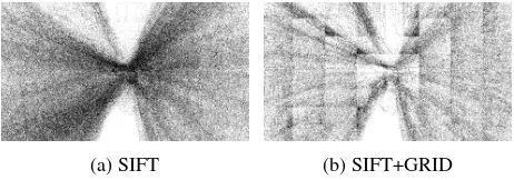
Due to rich textures in street scenes, thousands of interest points are usually detected in one image. We accumulate the locations of interest points in image sequence, hence a density map is gen-erated which indicates the probability of occurrence of interest points at the corresponding positions. Figure 1a depicts the den-sity of SIFT points computed with 89 images. It is obvious that most of the points are distributed around the image center.
(a) SIFT (b) SIFT+GRID
Figure 1. The density maps of interest points.
the center of images, the small parallax leads to inaccurate recon-struction of the points and consequently the poses parameters. On the other hand, the large number of points might decelerate the matching procedure and local bundle adjustment. A natural solu-tion is in dividing the images into cells, then limiting the number of detected feature points in each cell. This kind of methods have been widely used to get well distributed feature points (Zhang et al., 1995; Kitt et al., 2010). In this paper, a8×8pixel grid is used that divide each image into64cells. In each cell, the maximum number of the feature points is fixed as 32. Thus the most stable 32 feature points are kept if there are more than 32 feature points detected in one cell. If the number of detected feature points is less than 32, all of the points will be kept. The maximum num-ber of the detected feature points is64×32. The density of grid based SIFT is shown in figure 1b where more uniform distribu-tion of points is noticeable.
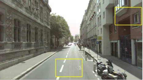
Figure 2. The interest points in the yellow rectangles are selected to show the difference from different extraction methods.
Figure 3 demonstrates the interest points on road and facades. The grid based methods enable to find more points in the non-central regions of the images. The close-up patches are shown as the rectangles in figure 2.
3.4 Matching
In our localization system, the pose of every frame in the se-quence is estimated, but only the key frames are kept, according to the moving distance. If the distance is larger than0.5m, the frame will be taken into account as key frame. In the matching process., we do not search the interest points in current frame with the points in all the previous key frames. In contrast, only latest three key frames are matched with the current frame. tis defined as the index for current image, the matching for imaget is to search the correspondences in the subsequence (t−1, t−
2, t−3). For each matching, the FLANN (Fast Library for Ap-proximate Nearest Neighbors) (Muja and Lowe, 2009) is used to search the correspondences. The euclidean distance between two description vectors of feature points in two frames is employed to measure the similarity. The distance ratio (T > 0.6) is ap-plied to filter the low quality matches. At last, the outliers are rejected using the epipolar constraint. An AC-RANSAC (A Con-trario RANSAC) (Moulon et al., 2013) based algorithm is used to estimate the fundamental matrix. Reject the matching results that the distances from image points to its corresponding epipolar lines are larger than2.0pixel.
4. THE PROCESS OF LOCALIZATION
Our localization approach assumes that the pose of first frame and the distance from first to second frame are known in advance. Then we estimate the initial values for poses and some 3D object points. Finally, the LBA is applied to optimize these parameters.
4.1 Initialization for image poses and object points
We define(R0, C0)as the pose of first image, whereR0is
rota-tion matrix from world to image andC0is the position of camera
center in world coordinate system. D is noted as the distance from first to second images. The pose of second image is
esti-mated by:
R1=RR0
C1=−D·R1ν
(1)
where,(R, ν)is the relative pose. TheRis rotation matrix and νis the transformation from first to second image. We estimate
(R, ν)using 5-point algorithm proposed by Nist´er (2004). Then, some 3D object points are computed by triangulation using the matched tie points between first and second images and the poses of first and second image. From third frame, the pose will be estimated using a set of 3D-2D correspondences derived from the alignment between the interest points in new image and the reconstructed 3D object points. A novel P3P (perspective-three-point) algorithm is used to solve the pose parameters (Kneip et al., 2011). The AC-RANSAC is employed to find the best estimates. With the newly estimated image pose, more 3D points can be reconstructed. The same procedure will be used to estimate the pose of other images and reconstruct more 3D points one by one.
4.2 Local bundle adjustment
Pose parameters are optimized by LBA (Mouragnon et al., 2006; Eudes and Lhuillier, 2009). Different with Global Bundle Adjust-ment (GBA) which aims to minimize the sum of squared back-projection errors (Triggs et al., 2000), LBA will minimize the back-projection errors under the constraint of prior posesC0
pin each sliding window, the cost function is shown in equation 3 .
argmin
C,X
1 2(v
T
t Wtvt+vTpQ− 1
Cpvp) (2)
and:
vp=Cp−Cp0
vt=F(Cp, Cn, Xt)−mt
where:
• Cn: the new image poses in current processing window.
• Cp: the prior poses inherited from previous steps.
• Xt: 3D points.
• F: projection function.
• mt: image points.
• vt: the vector of back-projection errors.
• vp: the vector ofCpresiduals.
• Wt: the weight matrix for image points.
• QCp: the covariance matrix ofCp.
• t: the index of frame.
In LBA,Cn, Cp, Xt are parameters andCn ={Ct−n+1...Ct} , Cp = {Ct−N−1...Ct−n}. TheN is the size of sliding
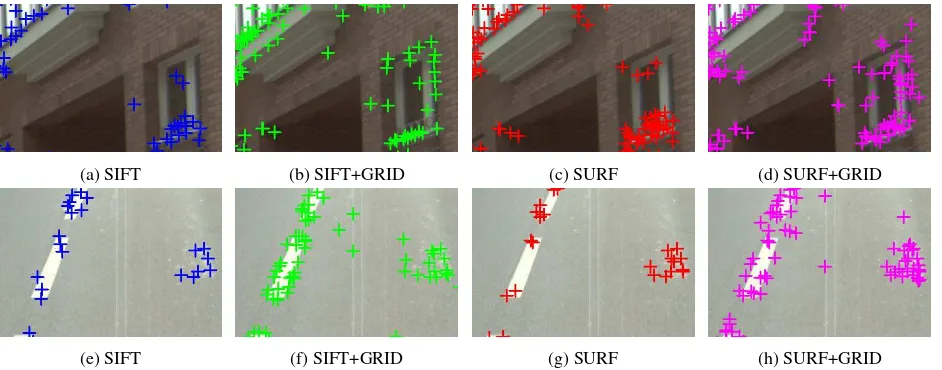
(a) SIFT (b) SIFT+GRID (c) SURF (d) SURF+GRID
(e) SIFT (f) SIFT+GRID (g) SURF (h) SURF+GRID
Figure 3. Some interest points are removed on road and facade for SIFT and SURF detectors. But the grid based SIFT or SURF detectors are able to keep these useful points for localization.
5. SETUP FOR THE EVALUATION 5.1 Repeatability
The repeatability is defined by the ratio between the number of correctly matched point pairs and the number of detected feature points (Schmid et al., 2000). In one image pair ([i, j]), the de-tected feature points are noted as:
{xk
i}k=1,...,Mi , {x m
j}m=1,...,Mj (3)
The correspondence between two points in the two images is noted asxk
i ∼ ǫ x
m
j with respect to the condition of homography transformation:
xki ∼ ǫ x
m
j ⇒dist(H·x k i −x
m
j )< ǫ (4)
whereHis homography matrix,ǫis the radius of neighborhood. The number of correspondences between imagesiandjwill be:
Φ(ǫ) = X
xk i∼ǫxmj
1 (5)
So the repeatability of interest points is defined as:
γ= Φ(ǫ)
min(Mi, Mj)
(6)
The value ofγprovides a good measure of repeatability for pla-nar scene in respect to homography transformation for one image pair. However, the matching in our localization system is a con-tinuous approach that each new image is matched with previous three images. So the aforementioned measurement of repeatabil-ity can not be suitable for us. Therefore, we consider the ratio between the number of tie points to the the number of feature points in each image as a new measure of repeatability. Tie point set is defined as:
{xi
t|dist(F(Cp, Cn, Xt)−xit)< ǫ} (7)
wherexi
t is a tie point in current imaget,ǫis the threshold for back-projection error which is set as3pixels in this paper. The number of interest points of imagetisMt, the repeatability cor-responding to imagetis :
ρ(t, ǫ) = |{x
i
t|dist(F(Cp, Cn, Xt)−xit)< ǫ}|
Mt
(8)
In this paper, the mean values ofρ(t, ǫ)is calculated to measure the repeatability. We assume the number of images isT, so the repeatability for the feature detector is calculated by:
ρ= 1
T ·
t<TX
t=0
ρ(t, ǫ) (9)
5.2 Posterior variance of interest points
In our approach, we estimate the variance of the feature points using Variance Component Estimation method (VCE). The co-variance matrix for the observations can be estimated by :
Q=σ02·Qe (10)
whereQis the variance matrix,σ2
0is the variance factor andQe
is the initial variance matrix. We assume all the interest points have the same detecting precision for each detector and setQeas identity matrix. Thus, the variance for the images points is equal toσ2
0. According to the theory of VCE, the variance factorσ 2 0
can be estimated by analyzing the residuals of the observations after bundle adjustment. The variance factor is estimated using the following equation (Luxen, 2003):
ˆ
σ0 2
=vˆ
T tvˆt
r (11)
where:
• ˆvtis the residual vector after adjustment.
LBA is an incremental approach and bundle adjustment is ap-plied in a local processing window. In this case, the VCE should be employed for each processing step and a number of variance factors are estimated for one dataset. Apart from this, the prior estimates of images poses in LBA are also a kind of observations in processing step. This strengthen the difficulty of using VEC in LBA. Furthermore, the precision of one interest point detector should be same for one dataset. Thus, global bundle adjustment is the only option for VCE. The observations for GBA are the interest points, the unknowns are the image poses and 3D object points. The residuals after bundle adjustment are only related to image points. So the posterior variance of image points can guide the quality of image points detection.
5.3 The accuracy of localization
The goal of our approach is to evaluate the performance of SIFT and SURF for localization. So the accuracy of localization is one of the most important criterion. The final results of localization can be impacted by the precision of detector, the stability of fea-ture points for matching and the distribution of the tie points. In order to make the criterion of localization accuracy comparable on trajectories with different lengths, the criterion is defined as the ratio between the absolute error of localization and the length of trajectory. The equation can be noted as:
et=
kZt−Zt0k
Lt
(12)
• Ztis the estimated image location .
• Z0
t is ground truth.
• Ltis the length of path from the beginning.
The numerator of equation 12 is the euclidean distance between the estimated position and ground truth. In this paper, the ground truth is acquired by a precise navigation system in our MMS.
5.4 Running time
For real time localization, the processing time is also an important criterion. We consider the running time from three aspects that are feature extraction, image matching and LBA. It is of couse the time for matching and LBA is highly related to the number of feature points. The computation time for LBA contains the time for initialization of the parameters and optimization.
6. RESULTS AND ANALYSIS 6.1 Dataset design
The data in this experiment were captured by STEREOPOLIS (Pa-paroditis et al., 2012). The ground truth for pose parameters is obtained by a precise navigation system. Images are captured by a calibrated front looking camera. The focal length of the camera is10mm, the image size is1920×1024pixels. The FOV of the camera is 70° in horizontal and 42° in vertical. Four datasets are designed for evaluation which are noted asD1, D2, D3, D4. The difference betweenD1, D2andD3, D4is the average sam-pling distance. The samsam-pling distance for first two sets (D1, D2) is about3mbut it is about6mforD3, D4. Table 1 shows the number of images and the length of each path.
Table 1. The number of images and the length of path for each dataset.
dataset D1 D2 D3 D4
number of images 91 89 87 106 length (m) 277 276 570 627
The pathsD1, D2, D3, D4are shown in figure 4.
(a)D1, D2 (b)D3, D4
Figure 4. The red dots are the locations of images and the images show the first view of the sequence.
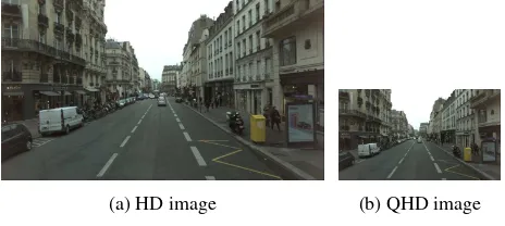
To test the impact of the image resolution, a sub-sampled set is generated for every original image dataset. The sub-sampled im-age sets are generated by resizing the imim-ages from original size (1920×1024) to960×512pixels. We note the original image as HD (High Definition) image and the sub-sampled image as QHD (Quarter High Definition). It is obvious that the number of de-tected points will be reduced in QHD image, so that the speed of localization will be improved. Figure 5 shows a sample of HD and QHD image.
(a) HD image (b) QHD image
Figure 5. HD and QHD image.
6.2 Evaluation measurements
The SIFT, SURF, SIFT+GRID and SURF+GRID are used to ex-tract the points of interest in HD and QHD images for every datasets. Thus, eight different types of results can be obtained for every datasets. Here the SIFT+GRID and SURF+GRID cor-respond to SIFT and SURF detectors applied with a grid adapter. The parameters for SIFT and SURF detectors are fixed for all the cases.
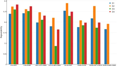
6.2.1 Repeatability of feature points: Figure 6a depicts the repeatability for the four datasets and theǫin equation 9 is set to
sampling distance. Therefore, it is more difficult to match the in-terest points inD3, D4. The previous investigation showed that SIFT outperforms SURF with the growing deformation caused by affine transformation (Juan and Gwun, 2009) between two im-ages. So SIFT can still be used in QHD+GRID case while SURF are failed to get enough matches.
The comparison between SIFT and SURF is made under same conditions (same resolution, constraint). In most of cases, SIFT shows better rate than SURF. For instance, the repeatability for HD+SIFT case is higher than HD+SURF and HD+SIFT+GRID is higher than HD+SURF+GRID.
Meanwhile, SIFT also shows its scale invariance. The repeatabil-ity rates are kept stable and even were improved a little bit from HD+SIFT to QHD+SIFT, but the repeatability for HD+SURF de-creases when sub-sampled images were used.
In addition, the repeatability decreases where the grid adapters are applied. As we discussed before, the feature points around image center can be easily matched between images, because of the small displacement of the pixel in center region in comparison with the pixel in the region out of center part where the view point changes are larger. If we reduce the points distributed in this re-gion, it also removes a large number of potential tie points. Com-pared with SURF, the SIFT provides better results. The decreas-ing for SIFT is smaller than SURF when grid adapter is used. Besides, SIFT would be a better option than SURF when pro-cess the large sampling distance image sequence. By observing the repeatability in HD+SIFT+GRID and HD+SURF+GRID, the repeatability values provided by SIFT forD1, D2, D3, D4are similar while the values forD3, D4using SURF are smaller.
6.2.2 Posterior variance of interest points: The posterior es-timated variances of the feature points are shown in figure 6b. Because of the same reason as previous section, the variance for QHD+SURF+GRID cannot be estimated with VCE.
The results in figure 6b tend to that SIFT still gives better per-formance than SURF. Because the variance for SIFT is smaller than SURF when they are used under same conditions. The vari-ances for SIFT method for all tested cases are less than 0.5 pixel while the variance for SURF detector is around 0.5 pixel and even larger. Apart form this, the diagram also depicts that the precision of the feature points for original images is slightly better than sub-sampling image by comparing the variance values in HD and QHD images for SIFT and SURF.
6.2.3 Accuracy of localization: The maximum error of lo-calization occurs at the last image in our approach and the values are shown in figure 6c for each method. The relative error of es-timated image positions is calculated with the method mentioned in section 5. and the results are shown in figure 6d. The state of the art visual odometry method can approach0.88%on the accu-racy of image position in KITT benchmark using stereo images (Cvii and Petrovi, 2015). We achieve around0.7%(Fig 6d) using HD+SIFT for all the four cases with monocular sequences. But we should mention that the resolution of our experimental images are higher than KITT datasets that the resolution is 1226×370 pixels.
The diagram depicts that the errors of position increase when the resolution of image changes from HD to QHD. Meanwhile, the grid adapter is not suitable for SURF especially for the large sampling distance cases (D3, D4). Both the maximum and rel-ative errors increase quickly if the grid adapter is used. The re-sult in both diagrams also reflect the robustness of SIFT, the er-rors keep flat for all the cases related to SIFT. We find that the
(a) Repeatability for each feature extraction method on different datasets.
(b) The posterior variance of interest points.
(c) The max errors of image position for different image sets. The lengths of path forD3, D4are longer thanD1, D2, so the maximal error of image position is large.
(d) The mean values of relative error for image position.
HD+SIFT+GRID is the most stable way among all the feature extraction strategies for localization, the relative error is less than one percent forD1, D2, D3, D4. Furthermore, HD+SIFT+GRID has more accurate localization results than HD+SIFT at most sets (D2, D3, D4). But this is not the case for SURF which leads to worse results when the grid adapter is applied. These figures also tend to illustrate the advantage of high resolution images where most of HD images can obtain better results than QHD with the same feature extraction method.
6.2.4 Runtime: Figure 6e shows the runtime for feature ex-traction, matching and LBA. Each part of localization procedure is demonstrated with different color of bin. The height of the bin represents the average processing time per image. It is ob-vious that the time spent on feature extraction and matching is much higher than LBA in our localization procedure from fig-ure 6e, where the blue and green bins are much higher than the red bins. In addition, the processing time can be reduced by subsampling the image (QHD) or limiting the number of fea-ture points (GRID). However, a trade-off between efficient and accuracy should be found. The SIFT and SURF used in this ex-periment are standard CPU based implementation. In the future, the feature extraction part can be speed up with GPU.
6.3 Further analysis
An accurate localization usually obtains low posterior variance and high repeatability. If the repeatability is too low, the local-ization may not be accurate. For instance, the repeatability for D3using HD+SURF+GRID is the very small (see Fig 6a), so the error of position is high in figure 6d.
Combining the results of repeatability, posterior variance and the accuracy, SIFT outperforms SURF on stability. For instance, the accuracy reduces too much when the resolution is decreased or the grid adapter is used, but SIFT performs better. In particular, the HD+ SIFT+GRID strategy achieves excellent results for all datasets, the posterior variances are almost the smallest (Fig 6b) in all the methods. Although the repeatability of HD+SIFT+GRID is slightly smaller than HD+SIFT, the localization accuracy is al-most the best. This indicates that the distribution of tie points is a more important factor than the large quantity of tie points.
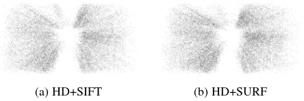
The posterior variance is relevant for evaluating the back projec-tion errors of the tie points. Thus the final estimaprojec-tion of pos-terior variance for the image points would be influenced by the accuracy of localization and precision of image point detection. As we discussed before, the distribution of tie points also im-pact the localization accuracy. However, if the same strategy is used for feature extraction, the distribution of tie points is simi-lar (cf. figure 7 which shows the accumulation map of HD+SIFT and HD+SURF). In this case, the posterior variance can reflect the precision of image points detector since the accuracies of the localization are equivalent. In figure 6d and 6c, the errors of HD+SIFT and HD+SURF are equivalent, but the posterior vari-ance of SURF is larger than SIFT in figure 6b. This phenomenon indicates that the SIFT detector is more precise than SURF in OpenCV implementation.
The HD+SURF performs slightly better than HD+SIFT for lo-calization accuracy. Even the distribution of the tie point for HD+SIFT and HD+SURF is very similar in figure 7, the quantity of tie points in the out of center area for SURF is higher where the intensity in figure 7b is darker than figure 7a. So there might be more reliable tie points in bundle adjustment.
(a) HD+SIFT (b) HD+SURF
Figure 7. The maps of tie points for HD images inD1. The image points are detected without GRID constraints.
7. CONCLUSION
An evaluation of SIFT and SURF for vision based localization was introduced in this paper. From our experiment, SURF was faster than SIFT on feature extraction, but SIFT was more reli-able considering the results from repeatability, precision and the accuracy of estimated poses. Therefore, SIFT might be more suit-able for our localization method. With the grid adapter, a better uniformly distributed interest points can be guaranteed. Thus we conclude that grid adapter (HD+SIFT+GRID) is the best option for us in localization approach.
In our experiments, the HD images have higher spatial resolu-tion than QHD images. Theoretically, HD image should obtain better localization accuracy. However, the posterior variance for HD+SIFT+GRID is only slightly better than QHD+SIFT+GRID while the absolute errors of localization are equivalent, as shown in figure 6d and 6b. This situation might mean that the tie point acquired from QHD+SIFT+GRID could be more stable and bet-ter distributed. But more investigation need to be done in this part. In order to take benefit from good distribution and precise 2D localization of tie points, one possible solution is to detect and match the interest points in QHD level, and re-localize the points in HD level. This kind of strategies have already been applied in some research(Bellavia et al., 2015). Besides, we should mention that some factors such as pose estimators, the triangulation preci-sion would also influence the localization accuracy. In the future work, more detailed experiments should be considered to include all of these factors. More advanced computing technologies such as GPU, application-specific integrated circuits (ASIC) or field-programmable gate arrays (FPGA) , can be considered to speed up the process.
ACKNOWLEDGE
we gratefully thank Val´erie Gouet-Brunet and David Vandergucht in MATIS Lab. for the discussions and suggestions about the feature extraction and matching.
REFERENCES
Agarwal, S., Mierle, K. and Others, n.d. Ceres solver. http: //ceres-solver.org.
Ballesta, M., Gil, A., Reinoso, O. and Mozos, O. M., 2007. Eval-uation of interest point detectors for visual slam. International Journal of Factory Automation, Robotics and Soft Computing 4, pp. 86–95.
Bay, H., Ess, A., Tuytelaars, T. and Van Gool, L., 2008. Speeded-up robust features (surf). Computer vision and image understand-ing 110(3), pp. 346–359.
Cvii, I. and Petrovi, I., 2015. Stereo odometry based on careful feature selection and tracking. In: Mobile Robots (ECMR), 2015 European Conference on, pp. 1–6.
Davison, A., 2003. Real-time simultaneous localisation and map-ping with a single camera. In: Computer Vision, 2003. Proceed-ings. Ninth IEEE International Conference on, pp. 1403–1410 vol.2.
Eudes, A. and Lhuillier, M., 2009. Error propagations for local bundle adjustment. In: Computer Vision and Pattern Recognition, 2009. CVPR 2009. IEEE Conference on, IEEE, pp. 2411–2418.
Gauglitz, S., H¨ollerer, T. and Turk, M., 2011. Evaluation of in-terest point detectors and feature descriptors for visual tracking. International journal of computer vision 94(3), pp. 335–360.
Grabner, M., Grabner, H. and Bischof, H., 2006. Fast approxi-mated sift. In: Computer Vision–ACCV 2006, Springer, pp. 918– 927.
Jiang, Y., Xu, Y. and Liu, Y., 2013. Performance evaluation of feature detection and matching in stereo visual odometry. Neuro-computing 120, pp. 380–390.
Juan, L. and Gwun, O., 2009. A comparison of sift, pca-sift and surf. International Journal of Image Processing (IJIP) 3(4), pp. 143–152.
Khan, N. Y., McCane, B. and Wyvill, G., 2011. Sift and surf performance evaluation against various image deformations on benchmark dataset. In: Digital Image Computing Techniques and Applications (DICTA), 2011 International Conference on, IEEE, pp. 501–506.
Kitt, B., Geiger, A. and Lategahn, H., 2010. Visual odometry based on stereo image sequences with ransac-based outlier re-jection scheme. In: Intelligent Vehicles Symposium (IV), 2010 IEEE, pp. 486–492.
Kneip, L., Scaramuzza, D. and Siegwart, R., 2011. A novel parametrization of the perspective-three-point problem for a di-rect computation of absolute camera position and orientation. In: Computer Vision and Pattern Recognition (CVPR), 2011 IEEE Conference on, IEEE, pp. 2969–2976.
Lowe, D. G., 2004. Distinctive image features from scale-invariant keypoints. International journal of computer vision 60(2), pp. 91–110.
Luxen, M., 2003. Variance component estimation in performance characteristics applied to feature extraction procedures. In: Pat-tern Recognition, Springer, pp. 498–506.
Mikolajczyk, K. and Schmid, C., 2005. A performance evaluation of local descriptors. Pattern Analysis and Machine Intelligence, IEEE Transactions on 27(10), pp. 1615–1630.
Moulon, P., Monasse, P. and Marlet, R., 2013. Adaptive structure from motion with a contrario model estimation. In: Computer Vision–ACCV 2012, Springer, pp. 257–270.
Mouragnon, E., Lhuillier, M., Dhome, M., Dekeyser, F. and Sayd, P., 2006. Real time localization and 3d reconstruction. In: Com-puter Vision and Pattern Recognition, 2006 IEEE ComCom-puter So-ciety Conference on, Vol. 1, IEEE, pp. 363–370.
Muja, M. and Lowe, D. G., 2009. Fast approximate nearest neigh-bors with automatic algorithm configuration. In: International Conference on Computer Vision Theory and Application VISS-APP’09), INSTICC Press, pp. 331–340.
Murillo, A. C., Guerrero, J. J. and Sagues, C., 2007. Surf features for efficient robot localization with omnidirectional images. In: Robotics and Automation, 2007 IEEE International Conference on, pp. 3901–3907.
Nist´er, D., 2004. An efficient solution to the five-point relative pose problem. Pattern Analysis and Machine Intelligence, IEEE Transactions on 26(6), pp. 756–770.
Nist´er, D., Naroditsky, O. and Bergen, J., 2004. Visual odometry. In: Computer Vision and Pattern Recognition, 2004. CVPR 2004. Proceedings of the 2004 IEEE Computer Society Conference on, Vol. 1, IEEE, pp. I–652.
Paparoditis, N., Papelard, J.-P., Cannelle, B., Devaux, A., Soheil-ian, B., David, N. and HOUZAY, E., 2012. Stereopolis ii: A multi-purpose and multi-sensor 3d mobile mapping system for street visualisation and 3d metrology. Revue franc¸aise de pho-togramm´etrie et de t´el´ed´etection (200), pp. 69–79.
Qu, X., Soheilian, B. and Paparoditis, N., 2015. Vehicle local-ization using mono-camera and geo-referenced traffic signs. In: 2015 IEEE Intelligent Vehicles Symposium (IV), pp. 605–610.
Saleem, S., Bais, A. and Sablatnig, R., 2012. A performance evaluation of sift and surf for multispectral image matching. In: Image Analysis and Recognition, Springer, pp. 166–173.
Schmid, C., Mohr, R. and Bauckhage, C., 2000. Evaluation of interest point detectors. International Journal of computer vision 37(2), pp. 151–172.
Schmidt, A., Kraft, M. and Kasi´nski, A., 2010. An evaluation of image feature detectors and descriptors for robot navigation. In: Computer Vision and Graphics, Springer, pp. 251–259.
Se, S., Lowe, D. and Little, J., 2001. Vision-based mobile robot localization and mapping using scale-invariant features. In: Robotics and Automation, 2001. Proceedings 2001 ICRA. IEEE International Conference on, Vol. 2, pp. 2051–2058 vol.2.
Strasdat, H., Montiel, J. M. and Davison, A. J., 2012. Visual slam: why filter? Image and Vision Computing 30(2), pp. 65–77.
Triggs, B., McLauchlan, P. F., Hartley, R. I. and Fitzgibbon, A. W., 2000. Bundle adjustmenta modern synthesis. In: Vision algorithms: theory and practice, Springer, pp. 298–372.
Valgren, C. and Lilienthal, A. J., 2010. Sift, surf & sea-sons: Appearance-based long-term localization in outdoor envi-ronments. Robot. Auton. Syst. 58(2), pp. 149–156.
Yang, Y., Song, Y., Zhai, F., Fan, Z., Meng, Y. and Wang, J., 2009. A high-precision localization algorithm by improved sift key-points. In: Image and Signal Processing, 2009. CISP ’09. 2nd International Congress on, pp. 1–6.