Global shocks and their impact on the Tanzanian economy

Received November 11, 2016 Published as Economics Discussion Paper November 24, 2016 Revised March 11, 2017 Accepted March 21, 2017 Published April 13, 2017

© Author(s) 2017. Licensed under the Creative Commons License - Attribution 4.0 International (CC BY 4.0)

Global shocks and their impact on the Tanzanian

economy

Fiseha Haile

Abstract

Plummeting commodity prices, China’s economic slowdown and rebalancing, and global financial market turbulence have recently raised concerns about their effects on African economies. This paper investigates whether, and to what extent, these intertwined shocks spillover into the Tanzanian economy. The author finds that a 1 percentage point (ppts) drop in China’s investment growth is associated with a decline in Tanzania’s export growth of roughly 0.60 ppts. A 1 percent fall in commodity prices leads to 0.65 percent lower exports value. The results suggest that a hard landing of the Chinese economy to its ‘new normal’ would doubtless send shock waves through the Tanzanian economy by further driving down commodity demand and prices as well as lowering development finance. In contrast, financial market volatility has a fairly negligible impact on economic growth. The main results stand up well to a wide-array of robustness checks.

JEL C32 F4 O11

Keywords China; Tanzania; commodity prices; investment; exports; Cointegrated VAR model

Authors

Fiseha Haile, World Bank, Addis Ababa, Ethiopia, fisehahaile77@yahoo.com

www.economics-ejournal.org 2

1

Introduction

Tanzania has posted high and sustained economic growth over the past decade, hovering around 6−7 percent. In addition, in recent years, inflation has been tamed to reasonable single digit levels. Tanzania has also maintained a broadly stable current account deficit. However, notwithstanding the overall positive short- to medium-term outlook (World Bank, 2016), the economy is not fully resilient to externally-induced shocks and, like many African economies, has recently been facing several growing and intertwined risks, including China’s economic slowdown, falling global commodity prices and, to a lesser extent, increased volatility in global financial and foreign exchange markets.

Over the past decade or so, trade and investment links between Tanzania and China have reached historically unprecedented levels. China is now one of Tanzania’s biggest trading partners and increasingly important source of development finance. However, although the increased economic ties are likely to have bolstered economic growth, they have doubtless increased Tanzania’s vulnerability to the vagaries of the Chinese economy. China’s investment-propelled growth seems to be running out of steam, partly reflecting rebalancing towards a consumption-driven and services-oriented economy (Lakatos et al., 2016).1 The structural shift has recently manifested itself in flagging demand and prices for commodities. China’s faltering growth may engender a significant knock-on effect on the Tanzanian economy via depressed export growth and potentially lower development finance.

Plummeting commodity prices also pose risks to Tanzania by virtue of its position as a primary exporter. Global commodity prices have generally been on a downward spiral mainly on account of falling demand in China and higher production capacity. The prices of Tanzania’s major export commodities, notably gold, are at record lows, despite a slight resurgence in recent months. This constituted the main factor underlying the country’s worsening terms-of-trade during the past few years. Falling oil prices have partly dampened the deterioration in the external balance as the country is a net importer of oil. However, the implications of soft commodity prices need to be carefully assessed given that a

1

www.economics-ejournal.org 3 wrong combination of price fluctuations (for instance, a continued decline in gold prices and rebounding oil prices) might put a dent in the country’s respectable growth.

Another cause for concern has been increased volatility in global financial and foreign exchange markets. Tanzania remained largely unscathed by previous financial market turbulences due to its limited financial development and global integration. However, since the country is drifting towards deeper financial integration, with rising private capital flows and external commercial borrowing as well as pending sovereign bond issuance, it has become increasingly prone to global market instabilities. A closer scrutiny thus seems warranted in light of surfacing concerns that increased global financial volatility might put a drag on Tanzania’s growth pace. Further, since the early 2015, the Tanzanian Shilling has seen significant depreciation on the back of a strong dollar appreciation and, to a limited extent, declining aid inflows. Hence the need for examining whether the sharp nominal depreciation has been associated with higher inflation.

The present paper is an attempt to explore whether, and to what degree, the aforementioned economic shocks spillover into the Tanzanian economy. Towards this end, we employ the Cointegrated VAR model as a statistical benchmark. The empirical estimates suggest that a 1 percentage point (ppts) decline in China’s investment growth is associated with 0.57 ppts decrease in Tanzania’s export growth. This underscores the importance of diversifying markets destination to mitigate headwinds from demand fluctuations. In addition, a 1 percent lower export commodity prices leads to a 0.65 percent decline in exports value, reflecting the fact that Tanzanian exports are predominated by less diversified and largely unprocessed primary commodities, and thus significantly prone to turbulences in commodity prices. Moreover, a 1 ppts increase in capital flow volatility would reduce economic growth by a negligible 0.01 ppts. Finally, the impact of a 1 percent depreciation of the nominal effective exchange rate is to increase the inflation rate by around 0.58 ppts, albeit offset by the inflation-reducing impacts of low oil and food prices.

www.economics-ejournal.org 4 The remainder of the paper is organized as follows: Section 2 discusses the main sources of external risks to the Tanzanian economy? Section 3 briefly presents the theoretical framework. Section 4 discusses the data, while Section 5 is devoted to empirical model specification. Section 6 discusses the empirical results. Finally, Section 7 winds up with concluding remarks.

2

External risks to the Tanzanian economy: An overview

Like many SSA economies, Tanzania has established unprecedented trade and investment links with China over the past decade or so; hence more vulnerable to China’s business cycle. In 2014, total Sino-Tanzania trade surged to about $2.6 billion from negligible levels in 2000. China is the third major export destination, absorbing about 13 percent of the country’s total exports. The bulk of Tanzania’s exports to China is accounted for by mineral and precious metal exports. The country’s exports plunged in the early 2010s due to a soft demand in China, although it somewhat rebounded in 2014 (Figure 1). Over the last decade, China’s unparalleled growth was mainly propped up by an investment boom, which in turn gave rise to soaring import demand for commodities and hence their prices. China’s shift from commodity-intensive investment-led growth to services-driven economy has thus depressed commodity demand, notably those for metals.2 Therefore, a contraction in exports is the primary transmission channel through which Tanzania may feel the impact of a slowdown in the Chinese economy.

A sharper-than-expected slowdown in China could also affect the Tanzanian economy via potentially lower development finance and FDI. China’s development loans to Tanzania have grown substantially over the past decade and have been instrumental in addressing the country’s severe infrastructure deficits. In the short-term, economic downturn in China seems less likely to have a dramatic impact on its economic engagement in Tanzania. However, themagnitude of the ripple effect in the future depends on how successful and smooth China’s economic rebalancing will be. To be sure, a hard landing of China’s economy to its ‘new normal’ would have a considerable negative impact on the Tanzanian economy via causing cutbacks in development finance.

The officially reported stock of Chinese FDI in Tanzania has increased more than six fold and was roughly estimated at $70 million in 2014, albeit still small in

2

www.economics-ejournal.org 5 absolute terms. If China’s economic growth loses it vigor, it may also put further strain on the Tanzanian economy through possible deceleration in FDI inflows. Tightening financial conditions in China could slow Chinese firms’ investments in Tanzania as they now draw funds from a shrinking pool. However, fluctuations in Chinese FDI are unlikely to send shockwaves through the economy as it makes up less than 1 percent of the total FDI stock. In addition, as China moves away from an investment-driven growth model, its state-backed firms may look for profitable opportunities abroad and Africa may be a prime destination considering that returns are large, competition is relatively limited, and the availability of cheap and plentiful labor.

The downward spiral in global commodity prices is another source of concern, which has been partly reinforced by China’s slowing growth trajectory. Despite the demand-driven surge in global commodity prices that started around 2002 and lasted more than a decade, often dubbed as the commodity “super-cycle”, prices

www.economics-ejournal.org 6 dropped steeply in recent years (Figure 2). The sharp slide in commodity prices has been instigated by weaker demand and higher production capacity. Oil prices witnessed a particularly large drop, reflecting resilient supply. Metal prices have also plummeted. Gold price, for instance, stood at $1,106 per ounce in March 2016, plunging nearly 75 percent from its peak in mid-2011. Tanzania’s gold exports fell dramatically from their peak of $2.3 billion in 2011/12 to around $1.3 billion in 2014/15. As Tanzania is a net oil importer, markedly lower oil prices have relieved its energy import bill. In fact, on the whole, the turbulence in commodity prices has not hitherto severely affected Tanzania. However, an unfortunate turn of events entailing, for instance, a significant drop in gold prices and a rebound in oil prices, would likely have an adverse impact on the country’s growth performance.

Low commodity prices might also negatively affect future outputs as their value is marked up or down with price changes. Tanzania has discovered vast reserves of natural gas and massive foreign investment is expected to flow to its near-shore gas sector. However, the persistent drop in the prices of oil and liquefied natural gas (LNG) could weigh on the sentiment of multinational companies and stifle investment in the short-term. Similarly, a drastic decline in mineral prices might lead to a scaling down of existing and new operations in the medium- to long-term.3

In addition, Tanzania may be affected by rising volatility in global financial markets. The recent bout of volatility spiked in the aftermath of heightened global risk aversion associated with the financial turbulence in China and somewhat bleaker prospects for emerging economies in general. Tanzania remained broadly unaffected by previous financial market turbulences due to its limited financial development and integration. However, as the county is gravitating towards deeper financial integration, with rising private capital flows and external commercial borrowing as well as pending sovereign bond issuance, it has become increasingly susceptible to global market instabilities. Net FDI inflows to Tanzania stood at $2.1 billion in 2014, from less than $400 million a decade ago (Figure 3), reflecting the country’s increasing reliance on potentially volatile private capital flows.4

Increased volatility in financial markets can affect Tanzania mainly by causing disruptions to capital flows.5 However, with FDI flows to Africa projected to

3

However, setting up investments in mining is expensive and hence operations that are underway would likely be reversed in the short- to medium-term only if prices fell short of variable costs. This, however, seems likely only in some mature investments.

4

In contrast, portfolio flows to Tanzania account for only a meager proportion of total private capital flows, testifying to the underdevelopment of the domestic capital market and restrictions on capital account transactions.

5

www.economics-ejournal.org 7 remain stable in the short-term (World Bank, 2015a), the impact of volatility in financial markets may be modest. If global volatility intensifies, however, the country could suffer from a slowdown or possible reversal of capital flows and uncertainties over future aid inflows. In recent years, low interest rates in international markets and subdued financial volatility have led a number of SSA economies to issue sovereign bonds. However, in the face of increasing global volatilities and US interest rates, Tanzania’s future plans to issue bonds are likely to entail higher costs

.

Turning to developments in the foreign exchange market, the Shilling depreciated sharply against the currencies of Tanzania’s major trading partners, except the Euro. As of January 2015, the nominal depreciation against the US dollar stood at nearly 30 percent year-on-year (see Figure 4). The large depreciation was mainly on account of strong dollar appreciation and, to a lesser extent, a decline in aid inflows. Despite the substantial Shilling depreciation, the inflation rate has been fairly stable and remained within single-digit levels. However, this does not necessarily imply that the former had no impact on inflation. The reason is that low and stable inflation could be the result of a confluence of counteracting factors. For example, falling oil prices might have neutralized the inflationary impact of currency depreciation. This necessitates untangling the impact of exchange rate movements on inflation.

3

Theoretical framework

3.1

China’s slowdown, commodity prices, and Tanzania’s exports

We are generally interested in addressing the central question of whether, and the extent to which, Tanzania is susceptible to China’s economic slowdown. In particular, the analysis attempts to quantitatively pin down trade spillovers from China’s potentially slower, and more balanced, growth into the Tanzanian economy. The impact of changes in China’s domestic investment on Tanzanian exports is examined based on a model that takes the following form6 (hereafter referred to as Model 1):

export_t =�₀+�₁cdit+�2price_t+�3y_tworld+�� (1)

∆export_t=�₀∗+�₁∗∆cdit+�2∗∆pricet+�3∗∆yt

world ₍₂₎

6

www.economics-ejournal.org 8 where export_t stands for Tanzania’s exports; cdi_t for China’s domestic fixed asset investment, which serves as a proxy for investment slowdown in China and the accompanying contraction in demand for Tanzania’s exports; price_t for Tanzania’s export commodity prices, included to capture the impacts on Tanzania’s exports of falling global commodity prices; y_tworld for world income, representing overall external demand for the country’s exports; and ∆ denotes the first difference operator. Eqs. (1) and (2) are estimated to quantify spillovers into Tanzania’s exports from an investment deceleration in China, which are measured by the key parameters: �1 and �1∗. As discussed in Section 4, the formulation of the

cointegrated VAR model allows us to estimate both the long-run (captured by �i in

Eq. (1)) and short-run (represented by �i∗ in Eq. (2)) effects of changes in the

respective explanatory variables. �1 and �1∗ are expected to be positive as higher

domestic investment in China tends to increase demand for Tanzania’s exports, with an additional impact operating through higher export prices. We expect �2 and �2∗ to be positive because higher export prices would translate into higher value of

exports. The coefficients likely represent causal relationships as it is highly implausible that the level of domestic investment in China and commodity prices are affected by Tanzania’s level of exports.

The focus is on domestic investment because it supposedly better captures China’s structural shift away from investment-driven growth and its potential economic slowdown. As touched upon previously, an investment boom underpinned China’s breakneck growth over the past decade and the ensuing rapid growth in import demand for primary commodities, which are the mainstay of Tanzania’s exports. In addition, China’s rebalancing towards a consumption-led economy is likely to be reflected in a slowdown in investment spending (Lakatos et al., 2016). IMF (2012) finds that economies within China’s supply chain and those with less diversified commodity exports are the most vulnerable to deceleration in China’s investment growth. Real output might serve as an alternative indicator of economic activity in China; however, it exhibits limited time variation compared to investment. Thus, investment may better help explain movements in exports, which vary substantially over time. However, as shown later in the paper, using output instead of investment leaves our main conclusion broadly unaffected. Note that we use total exports in nominal terms to capture both the volume and price effects on Tanzania’s exports of China’s domestic developments.7

7

www.economics-ejournal.org 9

3.2

Volatility in financial markets and growth

The contribution of capital flows to the Tanzanian economy and the impact of its volatility on GDP growth is assessed by estimating the following model (hereafter referred to as Model 2):

y_t =�₀+�₁cap_t+�₂invt+�3ext+�� (3)

∆y_t =�₀∗+�₁∗∆cap_t+�₂∗∆invt+�3∗∆ext+�4∆volt (4)

where y_t stands for Tanzania’s real GDP; cap_t for net private capital inflows to Tanzania, included to measure the contribution of international capital flows to national output and thus, by implication, the loss in real output associated with lower capital flows stemming from tightened global financial conditions; invt and

ext for domestic investment and exports respectively, which constitute additional

important determinants of real income; and ∆vol_� for the standard deviation of net capital flows and captures volatilities in capital flows.8

As noted above, capital flow is the main transmission mechanism through which turbulences in global financial markets might ripple into the domestic economy. Accordingly, perturbations to the economy arising from volatility in capital flows are modeled in Eq. (3) via the spillovers of changes in capital inflows into real national income and in Eq. (4) via the growth impact of capital flow volatility. �1 and �1∗ are expected to be positive because an increase in capital

inflows is widely believed to be beneficial to recipients through promoting productive investments, enhancing efficiency, and facilitating technology adoption. However, the impact of capital flows may also depend on their size and volatility, with flows being more beneficial to countries that have reached a certain threshold of financial and institutional development. We expect �2 and �3 to be positive for

obvious reasons. �4 is expected to be negative as capital inflow surges and

disruptive outflows carry risks to economies, particularly to low income countries like Tanzania.

3.3

Currency movements and inflation

The impact of changes in the nominal exchange rate on inflation is investigated based on the following model (hereafter referred to as Model 3):

8

www.economics-ejournal.org 10

∆p_t=�₀+�₁neert+�2∆poil_t +�3mt+�4∆p_tfood+�� (5)

where ∆p_� stands for the inflation rate; neer_� for nominal effective exchange rate (henceforth NEER);9∆p_�oil for world oil price inflation, controlling for the impact of supply shocks; m_� for broad money supply or M2, accounting for the effect of monetary policy shocks; and ∆p_�food for global food price inflation. �1 is the

parameter of particular interest and captures the effect of movements in NEER on inflation. A negative coefficient on �1 would be theoretically consistent as large

nominal depreciation (i.e. a decline in neer_�) triggers inflationary effects by, among others, increasing import prices. �3 > 0 suggests that an excessive growth in

aggregate demand induced by higher money supply increases domestic prices and fuel inflation, a phenomenon oft-described as ‘too much money chasing too few goods’. The coefficients on oil and food price inflation are also expected to be positive. Lower global oil and food prices have purportedly played a significant role in containing inflation within single-digits territory and might have partly offset currency depreciation-induced hikes in inflation. This is essentially an empirical question and needs to be settled based on thorough empirical analysis.

4

Data

4.1

China economic slowdown and commodity prices

The data are annual observations for the period 1990−2014 and comprise the variables: exports of goods and services (denoted with ex); China’s gross fixed capital formation (cdi); export price index (price); and world GDP (yworld). They are obtained from the World Bank’s World Development Indicators and the Bank of Tanzania. All variables except export are at constant market prices, i.e. they are adjusted for price (or inflation) effects. In addition, all data are given in US Dollars. We opt for the nominal value of exports; however, the main conclusion of this analysis is robust to using exports in constant prices instead. Looking at the effect on exports in constant prices would be tantamount to disregarding the impact of China’s economic slowdown operating via lower commodity prices. It bears noting that a valid assessment of the impact of China’s slowdown is difficult and somewhat premature because China’s strong economic ties with Tanzania are a relatively recent phenomenon. Thus, we focus on the period since 1990.

9

www.economics-ejournal.org 11 Although important variables are omitted from our analysis, this does not, in general, invalidate the long-run estimates. The reason is that cointegration property is invariant to changes in the information set, i.e. a long-run relation detected within a given set of variables will also be found in an enlarged variable set (Johansen, 2000). Note that we also estimate an extended model that includes net FDI flows to test the hypothesis that the level of FDI inflows to Tanzania is influenced by export commodity prices. The advantage of gradually expanding the information set is twofold. First, it greatly facilitates the identification of long-run relations. Second, it enables an analysis of the sensitivity of the results associated with the ceteris paribus assumption ingrained in the smaller model. The graphs of the variables in levels and first differences are shown in Appendix Figures 1 and 2, respectively.

4.2 Volatility in capital flows

The model linking capital flow volatility and economic growth is based on data spanning the period 1980–2014 and includes the following variables: real GDP (denoted with y_�); net private capital inflows (cap_t); exports of goods and services (ext); and gross domestic investment (invt). The data were extracted from the

World Bank’s World Development Indicators and IMF’s Balance of Payments Statistics. Because private capital inflows rose dramatically only over the past couple of decades, we check the robustness of the key findings by restricting the sample to cover only the period 1990–2014. However, focusing on the last two decades would likely increase the statistical significance of these variables. Appendix Figures 3 and 4 present the graphs of these variables both in levels and first differences, respectively.

4.3

Currency depreciation and inflation

For this analysis, we use monthly data for the period from January 2013 to January 2015 and include the variables: inflation rate (denoted with ∆p_�) (change in the log of consumer price index (CPI)); nominal effective exchange rate (neer_�); broad money or M2 (m_�); world oil price inflation (∆p_toil) (change in the log of crude oil price index); and global food price inflation (∆p_tfood). A broad monetary aggregate, such as M2, is likely to have a closer link with the inflation rate than base money.10

10

www.economics-ejournal.org 12 Nonetheless, the central bank can only control this broader aggregate indirectly by manipulating the monetary base. The analysis controls for the effects of monetary policy using broad money; however, using rather the monetary base or narrow money (M1− currency in circulation outside banks and demand deposits of Tanzanian residents with banks) does not significantly matter for the conclusions from this analysis.

Our analysis omits real GDP, a potential indicator for real economic activity because data on this variable are not available on a monthly basis. However, the key findings of the analysis would generally remain unchanged if we included real GDP for at least two reasons. First, due to invariance of cointegration analysis to expansions in the variable set, adding real GDP would leave the core (long-run) results from the smaller model more or less intact. Second, since our sample covers only the last three years and given overall economic activity was fairly stable during this period, higher (or lower) inflation rate seems less likely due to stronger (or weaker) economic growth and more likely due to increases (or declines) in global energy and food prices, less (or more) prudent monetary policy, and faster (or slower) depreciation of the Shilling (see World Bank, 2015b, 2016). The graphs of these variables in levels and first differences are shown in Appendix Figures 5 and 6, respectively.

5

Model specification

5.1

The Cointegrated VAR model

Macroeconomic time-series data are typically characterized by path dependence, interdependence, unit-root non-stationarity, structural breaks, as well as shifts in equilibrium means and growth rates. To be a satisfactory benchmark a statistical model needs to simultaneously address these data features. Path dependence would point to a time-dependent process such as the autoregressive model, variable interdependence to a system-of-equations approach, and unit-root nonstationarity to cointegration. The cointegrated VAR model satisfactorily deals with these salient features of the data. Unlike other approaches in which data are constrained in pre-specified directions and are assigned an auxiliary role of ‘quantifying’ the parameters of an ad hoc theoretical model, the cointegrated VAR methodology uses strict statistical principles to extract out meaningful relations from the data (Hoover et al., 2008; Spanos, 2009).

www.economics-ejournal.org 13 trends (the exogenous or pushing forces). The baseline model is specified with one lag, a linear trend restricted to the cointegration (long-run) relations and a number of dummy variables to be explained below:11

∆x_t=�β∗x∗_t−1+Γ₁∆x_t−1+ΦD_s,t+�D_i,t+�₀+�_t

where x_t∗₋₁=(�_t−1, t,t_��) is a p-dimensional vector of variables defined in Section 4;12 � represents adjustment (or error-correction) coefficients (denoting the speed of adjustment to equilibrium); β∗=(β′,β₁,β₁₁) is a vector of coefficients to the long-run relations; β′xt are r long-run relations; t is a linear trend (1,2,3,…), β₁ is a

r-dimensional vector of trend coefficients of the long-run relations; t_yy is a broken linear trend (…0,0,0,1,2,3,…) starting in the year yy and restricted to the long-run relations (see discussion below), β₁₁ measures the change in the linear trend coefficient (or slope) of the long-run relations that ensued the extraordinary event in yy;D_�,� is an unrestricted step dummy (0,0,0,1,1,1) starting in yy and controls for shifts in growth rates as well as changes in the means of long-run relations; D_i,� (…,0,0,0,1,0,0,0,…) is a permanent impulse dummy and accounts for an unanticipated one-period shock effects in yy; Φ and � are coefficients to the step and impulse dummies, respectively; �₀ is a vector of constant terms; �_� is a �× 1 vector of error terms; and ∆ is the first difference operator. Some of the variables in our models experienced significant breaks in their long-run trends (and thus mean-shift in their growth rates), which were modelled by allowing for a piecewise linear trend, β₁t+β₁₁t_��, in the long-run relations and a step dummy, D_s,t, in the equations, ∆x_�. Since all variables are in logs, their differences represent growth rates.

11

The software package OxMetrics (Doornik and Hendry 2001) was used to carry out all computations.

12

www.economics-ejournal.org 14

5.2

Specification tests

The VAR model is derived under the assumption of constant parameters and multivariate normality. Although parameter stability can be assessed using recursive test procedures, the small number of observations at our disposal circumscribes the power of available recursive procedures. However, since both parameter non-constancy and non-normal errors are often associated with periods of political and economic turbulence, such as supply shocks, war, severe droughts, civil unrest, and policy interventions, we improve parameter stability and mitigate on-normality by controlling for the most dramatic events using several dummy variables. In fact, some of the variables feature few extraordinarily large observations incongruous with the normality assumption.

First step in the empirical analysis is to determine the lag length of the VAR model. Statistical tests indicate that there is no evidence of residual autocorrelation in the VAR(1) (i.e. a model with a leg length of 1) for all models. Accordingly, the lag length was truncated to 1. However, the results obtained allowing for two lags are by and large similar with the ones presented below. Provided that there are no signs of autocorrelation in the residuals, and given the relatively large number of variables and small size of our sample, the VAR(1) model is a satisfactory and parsimonious representation of the variation in the data.

In Model 1, the following dates were classified as outlying observations: 1989, 1998, and 2009.13 These outliers correspond to observations with standardized residuals larger than 3.0, i.e. |� �⁄ _�|≥3.0, which is the standard criteria for identifying an outlier.14 An algorithm searching for breaks and aberrant observations developed in Doornik et al. (2013) was used to determine the existence, timing, and significance of outliers, and shifts in mean growth rates. The year 1989 corresponds to the sharp economic downturn in China due to civil unrest and the subsequent economic sanctions several countries imposed against it.15 1998 coincides with the decline in world commodity demand as a result of the Asian

13

Global oil and food price inflation, and world income were modelled as weakly (long-run) exogenous variables for two reasons. First, given the small size of the sample, we preserve degrees of freedom by treating these variables as exogenous. Second, it is highly implausible that the long-run paths of the variables are affected by any of the variables in our empirical models. However, the main results of this paper prove robust to relaxing this assumption.

14

Contrary to the case in static regressions, the dummies do not eliminate the corresponding observations. The dummies account for unanticipated shocks and given that these are no longer unanticipated in the next period, their lagged effects on the system are accounted for by the dynamics of the model.

15

www.economics-ejournal.org 15 financial crisis of 1997−1998, which led to a significant drop in Tanzania’s export prices. The year 2009 marks the global economic slump, also dubbed the Great Recession, which took a heavy toll on most advanced economies and saw world GDP drop by around 2 percent.

We also spotted a change in trend slope in (and thus a shift in the mean growth rate of) export price in 2002. As discussed in Section 2, global commodity prices moved onto higher growth trajectory in 2002, which lasted more than a decade and has often been referred to as commodities “super-cycle”. During this super-cycle period, Tanzania’s export prices experienced hefty growth. We control for this event using a broken linear trend in the long-run relations and a step dummy in the equations in 2002. The location shift in growth rates is shown in Appendix Figure 7. In sum, the specification for Model 1 includes a linear trend and a broken linear trend (with a change in trend slope in 2002) restricted to the long-run relations, an unrestricted shift dummy in 2002 (which controls for the shift in growth rates as well as the change in means of long-run relations), and an unrestricted impulse dummies (accounting for an unanticipated one-period shock effects) in 1998 and 2009.16 In addition, the baseline model treats world GDP as a weakly exogenous variable. (Appendix Table 3 shows that the key results are robust to relaxing this assumption.) Further, the lag length is set equal to k= 1 in levels.17

In Model 2, the diagnostic tests detected a structural break in real GDP in 2001 as well as a number of outlying observations. The former captures the relatively higher and sustained economic growth Tanzania enjoyed since the early 2000s (Appendix Figure 8). Average annual GDP growth exceeded 6 percent since 2001, which constitutes a remarkable break from the past, with growth averaging less than 3 percent during 1980–2000. Tanzania experienced a dramatic increase in investment in the second half of the 1980s following the adoption of the Economic Recovery Program, primarily fueled by surges in foreign aid inflows. The investment spikes in 1987 and 1990 were controlled for using impulse dummies. In addition, the observation 1985 was classified as ‘too large’, which is associated

16

The analysis controls for the most dramatic events using different types of dummy variables. For example, a shift in the equilibrium mean can be captured by a step dummy, �_���_�, defined as (0,…0,0,0,1,1,1,…,1), while a one-period shock effect can be accounted for by an impulse dummy, ����� , defined as (0,…,0,0,0,1,0,0,0,…,0). In addition, in models with changes in trend slopes in the long-run relations, there is a need to additionally account for the change in underlying trends (and thus the corresponding shift in long-run growth rates). Such events were modelled using a broken linear trends (���) in the long-run relations, �′�_�, and a step dummy (�_���_�) in the equations, ��. 17

www.economics-ejournal.org 16 with the sharp (relative) increase in net private capital inflows. In a nutshell, Model 2 was specified to allow for a linear trend and a broken linear trend (with a change in trend slope in 2001) restricted to the long-run relations, an unrestricted shift dummy in 2001 (which accounts for the mean shift in ∆�_� and controls for the shift in means of long-run relations), and an unrestricted impulse dummies in 1985, 1987, and 1990. In addition, statistical tests indicated that one lag was the optimal lag length and k was truncated to 1 accordingly.

Model 3 became well-specified when we allowed for a broken linear trend in 2013(7) (i.e. the seventh month of 2013) and 2014(8), and the impulse dummies: Di12.6t (where 12.6 denotes the sixth month of the year 2012),Di13.1t, and

Di13.4t. The trend break in 2013(7) represents the shift in the growth path of

inflation, which assumed astronomical proportions in 2012 and for most of 2013, whereas it receded to reasonable single-digit rates over the past two years and half. The broken trend in 2014(8) accounts for the change in the long-run trend underlying money supply. Money supply increased steeply until late 2014, after which it shifted to a noticeably lower growth path. See Appendix Figures 9 and 10. Further, there is evidence of considerable seasonality in the monthly data, which we accounted for using seasonal dummies. To sum up, the specification for Model 3 includes: a linear trend and broken linear trend (with changes in trend slope in 2013(7) and 2014(8)) restricted to the cointegration space, an unrestricted shift dummy in these periods, and an unrestricted impulse dummies in 2012(6), 2013(1), and 2013(4). In addition, the lag length for Model 3 was set equal to 2. Global food and oil price inflation rates were modeled as weakly exogenous variables in the baseline model.

We now shed some light on how the above-mentioned break points were identified and accounted for. As alluded to above, we identified the break dates based on a priori knowledge on the timing of special events, a graphical inspection of the data, as well as a statistical test for the presence of trend and level shifts in the data. The broken trend possesses the most significant coefficient at those periods and accordingly the models were specified with a change in trend slope at these points. The hypotheses that Tanzania has had no statistically significant shift in the mean growth rates of the series at the specified dates were strongly rejected (p-value: 0.00).

www.economics-ejournal.org 17 categorized as a growth turnaround it should be sustained for at least 8 years and the change in growth rate has to be at least 2 percentage points; (ii) A variables can experience more than one instance of growth turnaround as long as the dates are more than 5 years apart; (iii) Trend breaks were selected at 1% ‘target size’18 (i.e.

� = 0.01) in the Autometrics options in OxMetrics 7 (see Doornik et al., 2013). Note that we perform a sensitivity analysis to examine if the estimates based on the statistically and economically most credible break date are fairly robust to alternative candidate break points in the vicinity of the first-best break point. We find that the main conclusions of this paper prove robust to changes in the break dates.

In modelling structural breaks, the paper draws on the conventional (multivariate) cointegration approach in Johansen et al. (2000) and Hungnes (2010), which accommodates different types of structural breaks. Specifically, using such a multivariate framework, hypothesis testing on breaks in trend slopes (or shifts in growth rates) can be formulated and properly tested. A potential drawback of a system-of-equations approach is that the trend breaks are assumed to occur at the same date for all series. An alternative would be to use a univariate approach and apply some variant of the method proposed by Perron (1989). However, in our case, the use of a single equation model would be more restrictive and hard to justify in the face of overwhelming evidence for the existence of more than one cointegration relations in all three models. In addition, Bai et al. (1998) show that there are substantial gains in precision from using multivariate models in which several variables are modelled as cointegrated system. The use of multiple series sharpens inference about the existence and dates of shifts in the mean levels (Bai et al., 1998, pp. 420). In other words, a break in mean growth rates might be more readily detected and estimated in a multivariate setting including variables that are purportedly co-moving. In some respects, our approach is similar to that of Hausmann et al. (2005), Wacziarg and Welch (2008), and Jones and Olken (2008), who identify episodes of sustained shifts in growth rates and examine explanations for such transitions.

All empirical models inherently approximations of the actual data generating process and we now turn to assessing if the models described in the previous section are reasonable approximations. Table 1 reports multivariate specification test results as well as univariate statistic corresponding to normality tests for all three models under consideration. With the deterministic specifications and the dummies included, the models discussed above pass most of the specification tests

18

www.economics-ejournal.org 18 and describe the data reasonably well. No serious deviations from the assumptions of residual independence and normality was detected.

In the three models, the null of normal errors was only borderline accepted. However, a look at the univariate test statistic indicates that normality was accepted in all equations, albeit with a relatively small p-value for some of the variables due to excess kurtosis (long tails). This, coupled with the absence of autocorrelation, seems to suggest that the result of the multivariate test is a finite sample phenomenon given that we have a small sample and a large number of variables.19 A look at the univariate tests statistic in Table 1 clearly indicates that normality was borderline accepted due to excess kurtosis whereas all individual equations have a skewness close to zero. We have gone to great lengths to ensure a model set up where multivariate normality is accepted with a higher p-value by, inter alia, estimating a partial model conditioning on weakly exogenous variables and changing the sample period. All these avenues, however, lead to similar conclusions. The multivariate tests of no autocorrelation were not rejected in all except Model 1, although with relatively small p-values. Note that the main

Table 1. Model specification tests

Model 1 Model 2 Model 3

Var. p-value Var. p-value Var. p-value

Normality* 0.01 0.07 0.05

Ex 0.58 y 0.57 ∆p 0.39

CDI 0.07 Cap 0.16 neer 0.72

Price 0.54 Inv 0.14 m 0.12

Ex 0.08

Skewness Ex 0.09 y 0.40 ∆p 0.61

CDI 1.36 Cap 0.56 neer 0.00

Price 0.11 Inv 0.13 M 0.09

Ex 0.33

Excess kurtosis Ex 3.21 y 2.88 ∆p 3.56

CDI 5.02 Cap 4.56 neer 2.20

Price 3.81 Inv 3.53 m 4.63

Ex 4.29

Autocorrelation 0.09 0.11 0.17

ARCH 0.21 0.46 0.59

Note: These figures represent p-values. The p-values measure the degree to which the null hypothesis is accepted: The higher the p-value, the more strongly the null hypotheses of normal errors, no autocorrelation, and no ARCH effects are accepted. *The p-values in bold face correspond to tests of multivariate normality while those under the multivariate test results represent univariate tests statistic for each of the three models.

19

www.economics-ejournal.org 19 conclusions from our analysis prove robust to steps that might circumvent the problem, such as increasing the lag length. In addition, although there are some signs of moderate ARCH effects and excess kurtosis (long tails), cointegrated VAR results are reasonably robust to such effects (Gonzalo, 1994; Rahbek et al., 2002).

Having established an adequate statistical description of the data, the next step is determining the cointegration rank. The cointegration rank classifies the data into

� long-run relations towards which the process is adjusting (the pulling forces) and � − � relations which are pushing the process (the exogenous forces). The choice of rank is made based on a range of statistical criteria, such as the trace test, the largest unrestricted root of the characteristic polynomial for a given �, the t-ratios of the α coefficients for the ��ℎ _{cointegration vector, and the graphs of the}

��ℎ _{cointegration relation. Table 2 reports the p-values of the trace test (�), the} largest unrestricted characteristic root (�) and the largest �-value of the � coefficients (α ̂). The test results indicate that �∗ is the statistically mostcredible (first-best) choice of rank for all three models.20 This suggests that there exist two long-run relations among the variables in our models. The choice of rank is conventionally made based on the trace test.

However, because the trace test suffers from substantial power problem when the size of the sample is small, we also base the choice of rank on the significance of the � coefficients, the characteristic roots of the model, and the graphs of the long-run relations (Juselius, 2006: Chapter 8.5). For the choice of r=3, the largest unrestricted root for the three models seems a bit far from the unit circle whereas the t-values of � reveal that there is no significant adjustment to the last two cointegration vectors. In other words, the strong persistence and much less significant adjustment coefficients for the third cointegrating vector might be used as a safeguard against including it in the stationary part of the model. In addition, the graphs of the recursively calculated trace tests exhibit pronounced linear growth in the first two cointegration relations, but much less so in the last two, although the picture is not as clear cut for Model 3. Similarly, a glance at the graphs of the cointegration relations reveal that the last two cointegration vectors in Models 1 and 2, and the last three in Model 3 show distinct non-stationary behavior, pointing toward r = 2. Hence, taking all these into consideration, we consider the choice of r=2 to be a reasonable choice. It is important to note, however, that the main conclusions of this paper are fairly robust to altering the cointegration rank. See discussion in Section 6.

20

www.economics-ejournal.org 20

Table 2. Determination of cointegration rank

Trace test (�), characteristic roots (��), and t-values of � (��)

� �� ��

r∗−1 r∗ r∗+1 r∗−1 r∗ r∗+1 r∗−1 r∗ r∗+1 Model 1 (r∗ = 2) 0.07 0.39 0.57 0.83 0.67 0.67 3.2 3.4 1.7 Model 2 (r∗ = 2) 0.00 0.08 0.15 0.71 0.71 0.55 7.7 6.2 2.5 Model 3 (r∗ = 2) 0.00 0.01 0.04 0.83 0.72 0.50 4.4 5.7 2.1

Note: The figures represent p-values of the trace test (�), the largest unrestricted characteristic root (��), and the largest t-value of the error-correction coefficients (��).

6

Results

This section discusses the identified structures of long-run equilibrium relationships for Models 1 – 3. When interpreting the results in this section it should be borne in mind that a cointegration relation only measures the association between the variables over the long-run and as such does not say anything about causality. To say something about causality, we need to combine the cointegration coefficients, β, with the adjustment coefficients, �. For example, the hypothetical cointegration relation (x₁,�− �1x2,�)~�(0) describes a positive comovement between x₁,� and x2,�. If the adjustment coefficient�1, of x1,�, is negative and significant but the adjustment coefficient corresponding to x₂,� is insignificant, i.e.

�2= 0, we can say that the direction of causality runs form �2,� to �1,�, i.e.�1,� =

�1�2,�+��.

However, the interpretation becomes less straightforward in terms of sign effects as the number of variables in a long-run relation increases. As alluded to above, when discussing the empirical results below, it should be noted upfront that the small number of observations at our disposal circumscribes the power of some multivariate test statistic, such as the trace test and recursive tests of parameter stability. Thus, the results below need to be interpreted bearing in mind these caveats. In particular, considering the volatile history of Tanzania, some of the estimated coefficients may represent average historical effects.

6.1

China’s economic slowdown and commodity prices

www.economics-ejournal.org 21 unreliable results, which prompts the need for a statistical model that addresses this data feature. Further, omitted variables and multicollinearity problems could render the baseline estimates biased. Therefore, we also estimate the models using the cointegration VAR methodology. Unlike the OLS regression, collinearity between the variables does not result in imprecise estimates of the long-run relations based on the cointegrated VAR model. The reason for this is that, unlike the case with a regression analysis in levels, the cointegrated VAR formulation more or less circumvents the multicollinearity problem by transforming trending variables into stationary differences, ∆x_�, and stationary long-run relations, β′�_� (Juselius, 2006).

The baseline OLS results are reported in Columns 1 (long-run) and 4 (short-run) of Table 3. cdi_� possesses a positive coefficient estimate, suggesting that an increase in China’s domestic investment is associated with higher Tanzanian exports. A 1 percentage point (ppts) increase in China’s investment growth is correlated with 0.89 ppts increase in export growth. We now resort to the estimates from the cointegration analysis. Table 3 reports the identified structure of two long-run relations, which was accepted based on a high p-value of 0.74. The estimated structure is generically, empirically, and economically identified as defined in Johansen and Juselius (1994).

The first long-run relation is between exports value, China’s domestic investment, and prices. The estimated error-correction coefficients reveal that

Table 3. Impact of China’s slowdown and falling commodity prices (1990−2014)

Long-run analysis Short-run analysis

(1) (2) (3) (4)

OLS Cointegrated VAR

(Accepted with a p-value of 0.74)

Cointegrated

www.economics-ejournal.org 22 short-run adjustment occurs only through changes in exports, signifying its importance as an export long-run relationship

:

ex_� =0.57 cdi_�+0.65 price_�

T

he results suggest that ceteris paribus China’s domestic investment and export prices make positive contribution to long-run movements in exports. Specifically, the estimates, which represent causal effects, suggest that a 1 percent contraction in domestic investment in China would lead to a drop in Tanzania’s exports of about 0.57 percent. This is consistent with the fact that an investment boom buoyed up China’s impressive growth and that this was followed by burgeoning import demand for primary commodities, which account for the lion’s share of Tanzania’s export revenues. Conversely, the estimates reflect that a slower, more balanced, growth in China has depressed global demand for commodities and hence held back lower Tanzanian exports. The short-run results (Column 3 of Table 3) indicate that a 1 ppts decline in China’s investment growth is associated with 0.60 ppts decrease in Tanzania’s export growth.

The second long-run relationship describes a strong association between export prices, China’s domestic investment, and world income. The adjustment coeffi-cients show that only export price is error-correcting to this equilibrium relationship:

price_� =0.97 cdi_�+4.23 y_�world−0.30 t+0.11 t₂₀₀₂

We find that increases in China’s domestic investment and world income are associated with higher prices for Tanzania’s export commodities. The impact of a 1 percent investment slowdown in China is to reduce Tanzania’s export prices by nearly 1 percent. This is to be expected because Tanzania is one of the countries within China’s supply chain and a net exporter of commodities, the prices of which have been driven by China’s domestic economic developments for more than a decade.21 A case in point is the recent drop in China’s gold imports from Tanzania and the steady decline in the prices of gold over the last three years.22 In addition, we estimate that an additional 1 percent increase in world income is associated with an increase in export prices of about 4 percent. Vulnerability to wild fluctuations in world commodity prices remains to be the Achilles' heel of the

21

As noted previously, the commodities super-cycle in the 2000s and early 2010s, and the coming to an abrupt end of the seemingly-unstoppable surge in global commodity prices were partly triggered by swings in China’s business cycle.

22

www.economics-ejournal.org 23 Tanzanian economy. Needless to say, channeling efforts toward diversifying the export portfolio and markets destination, and improving the quality of existing products can help the country mitigate headwinds from price swings and thus boost its competitive standing. Altogether, the findings reflect the fact that Tanzania’s exports are mainly composed of less diversified commodities, the prices of which are generally determined in the global market and fall beyond the domains of Tanzanian policy makers.

These findings are sufficiently robust to a battery of sensitivity checks. Appendix Table 1 adds net FDI inflows to the data vector in Model 1 to examine how direct investment flows to Tanzania are affected by fluctuations in commodity prices. The results indicate that the first two long-run relations describe similar export and price relationships as in Model 1, consistent with the invariance of cointegration relations to expansions of the information set. The third long-run relationship indicates that commodity prices are among the key determinants of FDI inflows. Specifically, a 1 percent drop in export prices is associated with about 3 percent lower FDI inflows. This is to be expected as FDI flows to Tanzania have increasingly focused on export-oriented production mainly related to investments in extractive industries. Given that mineral and metal exports account for a good portion of Tanzania’s exports, a significant decline in their prices might lead to a scaling down of existing and new operations in the medium- to long-term.

As mentioned in Section 5, our baseline model specifies world income as a weakly (long-run) exogenous variable. Allowing world income to enter Model 1 as an endogenous variable, the analysis reaches the same conclusion as before (Appendix Table 3). In addition, Appendix Table 2 shows that the results based on the first-best choice of rank are robust to altering the cointegration rank to the second-best alternative of r = 3. Further, as the sample size is small, the use of dummies might have resulted in a considerable loss of degrees of freedom. Thus, we redo the analysis excluding all dummy variables (Appendix Table 2). Our key results remain broadly unchanged. Appendix Table 3 shows that the key conclusions also hold up well to using GDP instead of investment as an indicator for economic activity in China.

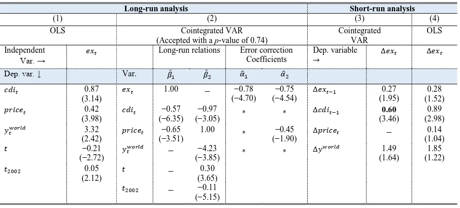
www.economics-ejournal.org 24 shock to be economically meaningful, the shock should purely represent an innovation to a particular variable instead of capturing a combined outcome of correlated errors. This would, however, require the causal structure of the model to be identified, rendering impulse responses susceptible to misinterpretation. Hence, we complement our impulse response analysis with statistical and economic evidence. In other words, we study the dynamic behavior of export following a one se shock to the above-mentioned variables. We find that the contemporaneous impact of a one se positive shock to domestic investment in China is an increase in Tanzania’s exports of about 0.05 percent. The large current impact is accompanied by a relatively modest increase, after which export gradually converges to its higher equilibrium level of about 1.2. Turning to the impact of shocks to export prices, the results show that export responds very slowly and the magnitude of the effect is quite small in the first few periods. This seems to suggest that export supply response to an increase in prices takes time to materialize. Following a shock to prices, export starts to increase steeply after few periods and thereafter converges smoothly to the long-run impact of 0.71 percent.

6.2 Volatility in capital flows

The OLS estimates in Column 4 of Table 4 show that higher volatility in capital flows has a statistically insignificant impact on economic growth. The baseline estimates are, however, valid only under fairly restrictive assumptions, which may not be borne out by the data. Thus, we turn to the results based on the cointegrated VAR model. For Model 2, the identified structure of two long-run relations was accepted based a quite high p-value of 0.97. Table 4 reports the results. Note that,

0

Figure 5. Impulse resonse of export

to a one SE shock to CDI

Figure 6. Impulse resonse of export to a

www.economics-ejournal.org 25

Table 4. Impact of volatility in capital flows (1980−2014)

Long-run analysis Short-run analysis

(1) (2) (3) (4)

OLS Cointegrated VAR

(Accepted with a p-value of 0.97)

Cointegrated

Note: t-values in parentheses. *Denote insignificant coefficients (�-value less than 1.80).

although two-long relations were detected, we focus on the first long-run equilibrium relationship, namely the GDP equation, because disentangling the contribution of private capital flows to the national economy and the growth impact of their volatility are of particular interest.

The first long-run relation comprises real GDP, net private capital inflows, and investment:

y_� =0.04 cap_�+0.26 inv_�+0.03 t₀₁

The estimated coefficients conform to a priori expectations. The results suggest that capital inflows have marginally significant positive contribution to national income. A 1 percent increase in net private capital inflows to Tanzania leads to a 0.04 percent increase in real GDP, which appears modest, albeit not negligible. The positive impact of capital flows is in line with economic theory as capital inflows are widely believed to benefit host countries through, inter alia, fostering productive investments, unleashing efficiency, and accelerating the transfer of technology. The small impact may be partly due to the fact that FDI flows, which account for nearly all of the total private capital inflows to the country, grew considerably only recently and that it may take a while before they translate into higher level of output.

www.economics-ejournal.org 26 impact on economic growth in Tanzania. In particular, a 1 ppts increase in the volatility of net private capital inflows reduces growth by 0.01 ppts. The quite modest effect seems to reflect the very small proportion of portfolio capital flows, which tend to be more volatile and susceptible to changes in global financial markets compared with FDI. The conventional wisdom suggests that, despite theoretically sound arguments in favor of private capital flows, portfolio equity and debt flows may pose substantial countervailing risks for developing economies as they are often motivated by speculative considerations and thus prone to quick reversals (Reinert et al., 2010). In Hausmann and Fernández-Arias (2000), short-term capital flows are referred to as “bad cholesterol”. In contrast, FDI is chiefly driven by long-term prospects and relatively irreversible in the short-run; hence considered “good cholesterol”. Many developing countries, including Tanzania, consider FDI as the private capital inflow of choice due to its purported resilience in times of financial turbulence. This is in line with the growing consensus that low income countries may need to reach a certain level of financial and institutional development before they can start reaping the potential benefits of ‘relatively’ unfettered capital flows.

6.3 Currency depreciation and inflation

The baseline OLS estimates are reported in Column 1 of Table 5. We find that a 1 percent nominal exchange rate depreciation is associated with a higher inflation rate of around 0.3 ppts. Moreover, money supply is negatively linked with inflation, which appears counterintuitive at first glance. However, the estimated coefficient does not represent causal relationship and likely captures the tendency of the central bank to reduce money supply when inflation soars.

The identified long-run structure for Model 3 is shown in Column 2 of Table 5, which was accepted based on a very high p-value of 0.93. Only the inflation equation is discussed below as the overriding objective of the analysis is to examine the impact of currency depreciation on inflation. The long-run relation for the inflation rate is given by:

∆p_� =−0.58 neer_�+0.21 ∆p_�oil+0.51 ∆p_�food+ 0.02t13(7)

www.economics-ejournal.org 27

Table 5. Nominal currency movements and inflation (Jan. 2013–Jan. 2015)

OLS Cointegrated VAR

(Accepted with a p-value of 0.93)

(1) (2)

Note: t-values in parentheses. *Denote statistically insignificant adjustment coefficients (�-value less than 1.80).

inflation in Tanzania. Specifically, a 1 percent depreciation of the NEER leads to 0.58 ppts higher inflation. In addition, global oil and food price inflation rates constitute important drivers of domestic inflation. A 1 ppts fall in global oil and food price inflation rates results in lower inflation of about 0.21 ppts and 0.51 ppts, respectively. The analysis finds no statistically significant link between changes in money supply and inflation. Relaxing the assumption that oil and food price inflation were exogenously determined does not significantly affect the baseline findings.

www.economics-ejournal.org 28 depreciation has no significant contemporaneous and one-period lagged impact on inflation, a result corroborated by findings from impulse response analysis. This is not too surprising as the analysis focuses on a sample covering only three years and relatively high-frequency monthly data, which might suggest that it takes more than one month for a sizable nominal depreciation of the Shilling to take effect.

7

Concluding remarks

This paper conducted a thorough empirical analysis of the macroeconomic impacts of recent global economic shocks in Tanzania. In particular, we set out to address the intertwined questions of whether, and to what extent, China’s economic slowdown, falling global commodity prices, and volatility in financial and foreign exchange markets spillover into the Tanzanian economy. The analysis uses the Cointegrated Vector Autoregressive (VAR) model as a statistical benchmark and is generally based on data spanning the period 1980–2015.

We find a strong evidence to suggest that China’s structural rebalancing away from commodity-intensive investment-led economy and its waning economic growth are associated with a significant contraction in Tanzania’s exports. The empirical estimates indicate that a 1 percentage point (ppts) lower investment growth in China is linked with 0.6 ppts decline in Tanzania’s export growth. In addition, long-run analysis revealed that a 1 percent contraction in China’s domestic investment would lead to a drop in Tanzania’s exports of about 0.57 percent. These findings do not come as much of a surprise considering that China is now the country’s third major export destination, with total Sino-Tanzania trade surging to around $2.6 billion in 2014 from negligible levels in the early 2000s. The rapidly increasing importance of China’s development finance to Tanzania indicates that a slowing Chinese economy might put further strain on the domestic economy via lower development loans and, to a limited extent, aid. However, lower Chinese FDI is unlikely to trigger sweeping repercussions on the economy since it accounts for just less than 1 percent of the total FDI stock in Tanzania, among other factors.

www.economics-ejournal.org 29 emerging market economies, the country may need to make concerted endeavors to diversify export destinations.

In addition, we found that a 1 percent fall in export prices is associated with a 0.62 percent decrease in exports value. This attests that vulnerability to the vagaries of world market prices remains to be the Achilles' heel of the Tanzanian economy. Therefore, efforts targeted at diversifying the export portfolio and improving the quality of existing products can help the country mitigate headwinds due to price fluctuations and strengthen its external competitiveness.

The empirical results also suggest that a 1 percent increase in net private capital flows to Tanzania contributes about 0.04 percent to national income while capital flow volatility barely reduces growth by 0.01 ppts. The very modest impact of increased volatility in capital flows is not too surprising given Tanzania has relatively low level of financial development and shallow integration into the global economy. Tanzania has so far opted for FDI over short-term portfolio equity and debt flows, which partly explains why the country has generally remained unscathed by previous global financial turbulences. However, as the economy is moving towards deeper financial integration, with rising private capital flows and external commercial borrowing as well as pending sovereign bond issuance, a significant rise in financial market volatility may pose substantial risks in the future.

Finally, faster nominal currency depreciation is associated with higher inflation in Tanzania. Specifically, a 1 percent depreciation of the nominal effective exchange rate leads to 0.58 ppts higher inflation rate. In addition, the impact of a 1 ppts drop in world oil and food price inflation rates would be to reduce overall domestic inflation by 0.2 ppts and 0.5 ppts, respectively. Therefore, despite the considerable depreciation of the Tanzanian Shilling since the early 2015, the inflation rate has remained low and stable mainly due to the countervailing effects of extraordinarily low import prices, notably that of oil. The main findings of this paper have been shown to be sufficiently robust to a battery of sensitivity checks.

www.economics-ejournal.org 30

References

Bai J., R.L. Lumsdaine, and J.H. Stock (1998). Testing for and Dating Common Breaks in Multivariate Time Series. Review of Economic Studies 65(3): 395–432.

https://academic.oup.com/restud/article-abstract/65/3/395/1565347/Testing-For-and-Dating-Common-Breaks-in

Doornik, J.A., and D.F. Hendry (2001). Empirical Econometric Modelling Using PcGive, Volumes I, II and III. London: Timberlake Consultants Press.

Doornik, J.A., D.F. Hendry, and F. Pretis (2013). Step-Indicator Saturation. Discussion Paper 658, Department of Economics, University of Oxford.

https://www.economics.ox.ac.uk/Department-of-Economics-Discussion-Paper-Series/step-indicator-saturation

Drummond, P., and E.X. Liu (2013). Africa’s Rising Exposure to China: How Large are Spillovers through Trade? IMF Working Paper No. 250. IMF, Washington, D.C.

https://www.imf.org/external/pubs/cat/longres.aspx?sk=41144.0

Gonzalo, J. (1994). Five Alternative Methods of Estimating Long-run Equilibrium Relationships. Journal of Econometrics 60(1-2): 203–233.

http://www.sciencedirect.com/science/article/pii/0304407694900442

Hausmann, R., and E. Fernandez-Arias (2000). Foreign Direct Investment: Good Cholesterol? RES Working Papers No. 417. Washington, D.C.: Inter-American Development Bank.

https://pdfs.semanticscholar.org/c911/70e74fba30c38f19bf977adb1a40165f896b.pdf

Hausmann, R., L. Pritchett, and D. Rodrik (2005). Growth Accelerations. Journal of

Economic Growth 10(4): 303–329.

http://link.springer.com/article/10.1007/s10887-005-4712-0

Hoover, K., K. Juselius, and S. Johansen (2008). Allowing the Data to Speak Freely: The Macroeconometrics of the Cointegrated Vector Autoregression. American Economic

Review 98(2): 251–255.

https://ideas.repec.org/a/aea/aecrev/v98y2008i2p251-55.html

Hungnes, H. (2005). Identifying the Deterministic Components in GRaM for Ox Professional: User Manual and Documentation. Mimeo.

http://www.hungnes.net/GRaM

Hungnes, H. (2010). Identifying Structural Breaks in Cointegrated Vector Autoregressive Models. Oxford Bulletin of Economics and Statistics 72(4): 551–565.

http://onlinelibrary.wiley.com/doi/10.1111/j.1468-0084.2010.00586.x/abstract

IMF (2012). China: Chapter IV Spillover Report, July 2012. Washington, D.C.: IMF.