getdocd080. 883KB Jun 04 2011 12:05:00 AM

(1)

El e c t ro n ic

Jo ur n

a l o

f

P r

o b

a b i l i t y

Vol. 11 (2006), Paper no. 24, pages 585–???.

Journal URL

http://www.math.washington.edu/~ejpecp/

Renormalization analysis of catalytic Wright-Fisher

diffusions

Klaus Fleischmann∗ Weierstrass Institute for Applied

Analysis and Stochastics Mohrenstr. 39 D–10117 Berlin, Germany

e-mail: fleischm@wias-berlin.de URL: http://www.wias-berlin.de/˜fleischm

Jan M. Swart† ´

UTIA

Pod vod´arenskou vˇeˇz´ı 4 18208 Praha 8 Czech Republic

e-mail: jan.swart@uni-tuebingen.de URL: http://staff.utia.cas.cz/swart/

Abstract

Recently, several authors have studied maps where a function, describing the local diffusion matrix of a diffusion process with a linear drift towards an attraction point, is mapped into the average of that function with respect to the unique invariant measure of the diffusion process, as a function of the attraction point. Such mappings arise in the analysis of infinite systems of diffusions indexed by the hierarchical group, with a linear attractive interaction between the components. In this context, the mappings are called renormalization transformations. We consider such maps for catalytic Wright-Fisher diffusions. These are diffusions on the unit square where the first component (the catalyst) performs an autonomous Wright-Fisher diffusion, while the second component (the reactant) performs a Wright-Fisher diffusion with a rate depending on the first component through a catalyzing function. We determine the limit of rescaled iterates of renormalization transformations acting on the diffusion matrices of such catalytic Wright-Fisher diffusions

∗_{Work sponsored through a number of grants of the German Science Foundation, and by the Czech Science} Foundation (GAˇCR grant 201/06/1323)

(2)

Key words: Renormalization, catalytic Wright-Fisher diffusion, embedded particle system, extinction, unbounded growth, interacting diffusions, universality

(3)

Part I

1 Introduction and main result

(4)

bulk of this paper is devoted to the proof of one theorem (Theorem1.4) about one transformation (defined in (1.2)), we come back to the relevance of our work for interacting diffusions in the discussion in Section 4and in an appendix.

Several authors [BCGdH95, BCGdH97, dHS98, Sch98, CDG04] have studied maps where a function, describing the local diffusion matrix of a diffusion process, is mapped into the average of that function with respect to the unique invariant measure of the diffusion process itself. Such mappings arise in the analysis of infinite systems of diffusion processes indexed by the hierarchical group, with a linear attractive interaction between the components [DG93a,DG96, DGV95]. In this context, the mappings are called renormalization transformations. We follow this terminology. For more on the relation between hierarchically interacting diffusions and renormalization transformations, see AppendixA.1.

Formally, such renormalization transformations can be defined as follows.

Definition 1.1 (Renormalization class and transformation) Let D ⊂Rd _{be nonempty,}

convex, and open. Let _W be a collection of continuous functionsw from the closureDinto the space Md

+ of symmetric non-negative definite d×dreal matrices, such that λw ∈ W for every λ >0,w∈ W. We call W a prerenormalization classon Dif the following three conditions are satisfied:

(i) For each constantc >0,w_{∈ W}, andx_∈D, the martingale problem for the operatorAc,wx is well-posed, where

Ac,w_x f(y) :=c d X

i=1

(xi−yi)_∂y∂_if(y) + d X

i,j=1

wij(y) ∂ 2

∂yi∂yjf(y) (y∈D), (1.1)

and the domain ofAc,wx is the space of real functions onDthat can be extended to a twice continuously differentiable function on Rd _{with compact support.}

(ii) For each c > 0, w _{∈ W}, and x _∈ D, the martingale problem for Ac,wx has a unique stationary solution with invariant law denoted byνxc,w.

(iii) For each c >0,w_{∈ W},x_∈D, and i, j= 1, . . . , d, one has Z

D

ν_xc,w(dy)_|wij(y)|<∞.

If W is a prerenormalization class, then we define for eachc > 0 and w∈ W a matrix-valued functionFcwon Dby

Fcw(x) := Z

D

ν_xc,w(dy)w(y) (x_∈D). (1.2)

We say that W is arenormalization classon D if in addition:

(iv) For eachc >0 andw_{∈ W}, the functionFcwis an element of W.

If_W is a renormalization class and c >0, then the mapFc :W → W defined by (1.2) is called

the renormalization transformation on W with migration constant c. In (1.1), w is called the

(5)

Remark 1.2 (Associated SDE) It is well-known that D-valued (weak) solutions y = (y1, . . . ,yd) to the stochastic differential equation (SDE)

dyi_t=c(xi−yti)dt+ √

2 n X

j=1

σij(yt)dBtj (t≥0, i= 1, . . . , d), (1.3)

where B = (B1, . . . , Bn) is n-dimensional (standard) Brownian motion (n ≥ 1), solve the martingale problem for Ac,wx if the d×n matrix-valued function σ is continuous and satisfies P

kσikσjk =wij. Conversely [EK86, Theorem 5.3.3], every solution to the martingale problem forAc,wx can be represented as a solution to the SDE (1.3), where there is some freedom in the

choice of the rootσ of the diffusion matrixw. ✸

In the present paper, we concern ourselves with the following renormalization class on [0,1]2.

Definition 1.3 (Renormalization class of catalytic Wright-Fisher diffusions) We set

Wcat:={wα,p :α >0, p∈ H}, where

wα,p(x) :=

αx1(1−x1) 0

0 p(x1)x2(1−x2)

(x= (x1, x2)∈[0,1]2), (1.4)

and

H:={p:pa real function on [0,1], p≥0, p Lipschitz continuous}. (1.5) Moreover, we put

Hl,r :=_{p_{∈ H}: 1_{p(0)>0}=l, 1_{p(1)>0} =r_} (l, r= 0,1), (1.6) and set_W_catl,r :=_{wα,p:α >0, p_{∈ Hl,r}_} (l, r= 0,1). ✸

Note that we do notrequire thatp >0 on (0,1) (compare the remarks below Lemma2.4). By Remark1.2, solutionsy= (y1_,_y2_{) to the martingale problem for}_Ac,wα,p

x can be represented as solutions to the SDE

(i) dy_t1=c(x1−yt1)dt+ q

2αy1

t(1−y1t)dBt1, (ii) dy_t2=c(x2−yt2)dt+

q 2p(y1

t)y2t(1−y2t)dBt2.

(1.7)

We cally1 the Wright-Fishercatalystwithresampling rateα andy2 the Wright-Fisherreactant

withcatalyzing functionp.

For any renormalization class W and any sequence of (strictly) positive migration constants (ck)k≥0, we define iterated renormalization transformationsF(n) :W → W, as follows:

F(n+1)w:=Fcn(F

(n)_w) _(n_≥₀₎ _with _F(0)_w_:=_w _(w_{∈ Wcat).} _(1.8)

We set s0 := 0 and

sn:= n−1 X

k=0 1 ck

(1_≤n_{≤ ∞}). (1.9)

(6)

Theorem 1.4 (Main result)

(a)The set _Wcat is a renormalization class on [0,1]2 _and _F

c(Wcatl,r)⊂ Wcatl,r (c >0, l, r= 0,1).

(b) Fix (positive) migration constants(ck)k≥0 such that

(i) sn_n→∞−→ ∞ and (ii) sn+1 sn n→∞−→

1 +γ∗ (1.10)

for some γ∗ ≥0. If w∈ Wcatl,r (l, r= 0,1), then uniformly on [0,1]2,

snF(n)w −→ n→∞w

∗_, _(1.11)

where the limit w∗ is the unique solution in Wcatl,r to the equation

(i) (1 +γ∗)F1/γ∗w∗=w∗ if γ∗ >0,

(ii) 1₂ 2 X

i,j=1

w∗_ij(x)_∂x∂2

i∂xjw

∗_{(x) +}_w∗_{(x) = 0} _(x

∈[0,1]2) if γ∗ = 0. (1.12)

(c) The matrix w∗ is of the form w∗ =w1,p∗

, where p∗ =p∗_l,r,γ∗ ∈ Hl,r depends on l, r, and γ∗.

One has

p∗_0,0,γ∗ ≡0 and p_1,1,γ∗ ∗ ≡1 for allγ∗ ≥0. (1.13)

For each γ∗ ≥ 0, the function p_0,1,γ∗ ∗ is concave, nondecreasing, and satisfies p∗_0,1,γ∗(0) = 0,

p∗_0,1,γ∗(1) = 1. By symmetry, analoguous statements hold for p∗_1,0,γ∗.

Conditions (1.10) (i) and (ii) are satisfied, for example, for ck = (1 +γ∗)−k. Note that the functions p∗_0,0,γ∗ and p∗_1,1,γ∗ are independent of γ∗ ≥ 0. We believe that on the other hand,

p∗_0,1,γ∗ is not constant as a function of γ∗, but we have not proved this.

The functionp∗_0,1,0 is the unique nonnegative solution to the equation 1

2x(1−x) ∂2

∂x2p(x) +p(x)(1−p(x)) = 0 (x∈[0,1]) (1.14) with boundary conditions p(0) = 0 and p(1)>0. This function occurred before in the work of Greven, Klenke, and Wakolbinger [GKW01, formulas (1.10)–(1.11)]. In Section 4.1 we discuss the relation between their work and ours.

Outline In Part I of the paper (Sections 1–4) we present our results and our main techniques for proving them. Part II (Sections 5–9) contains detailed proofs. Since the motivation for studying renormalization classes comes from the study of linearly interacting diffusions on the hierarchical group, we explain this connection in AppendixA.

(7)

Notation If E is a separable, locally compact, metrizable space, thenC(E) denotes the space of continuous real functions on E. If E is compact then we equip C(E) with the supremum norm _{k · k∞}. We let B(E) denote the space of all bounded Borel measurable real functions on E. We write C+(E) and C[0,1](E) for the spaces of all f ∈ C(E) with f ≥ 0 and 0 ≤ f ≤ 1, respectively, and define B+(E) and B[0,1](E) analogously. We let M(E) denote the space of all finite measures on E, equipped with the topology of weak convergence. The subspaces of probability measures is denoted by M1(E). We write N(E) for the space of finite counting measures, i.e., measures of the formν =Pm

i=1δxi with x1, . . . , xm ∈E (m ≥0). We interpret

ν as a collection of particles, situated at positions x1, . . . , xm. For µ ∈ M(E) and f ∈ B(E) we use the notation _hµ, f_i :=R

Efdµ and |µ|:= µ(E). By definition, DE[0,∞) is the space of cadlag functionsw: [0,∞)→E, equipped with the Skorohod topology. We denote the law of a random variableyby_L(y). Ify= (yt)t≥0 is a Markov process inE andx∈E, thenPx denotes the law of y started in y0 = x. If µ is a probability law on E then Pµ denotes the law of y started with initial lawL(y0) =µ. For time-inhomogeneous processes, we use the notationPt,x orPt,µ to denote the law of the process started at timet with initial stateyt=x or initial law L(yt) =µ, respectively. We let Ex, Eµ, . . . etc. denote expectation with respect toPx, Pµ, . . ., respectively.

AcknowledgementsWe thank Anton Wakolbinger and Martin M¨ohle for pointing out reference

[Ewe04] and the fact that the distribution in (5.17) is aβ-distribution. We thank the referee for a careful reading of an earlier version of the manuscript.

2 Renormalization classes on compact sets

2.1 Some general facts and heuristics

In this section, we explain that our main result is a special case of a type of theorem that we believe holds for many more renormalization classes on compact sets in Rd_{. Moreover, we}

describe some elementary properties that hold generally for such renormalization classes. The proofs of Lemmas 2.1–2.8can be found in Section5.1 below.

Fix a prerenormalization class _W on a set D where D _⊂ Rd _{is open, bounded, and convex.}

Then W is a subset of the cone C(D, M₊d) of continuous M₊d-valued functions onD. We equip C(D, M₊d) with the topology of uniform convergence. Our first lemma says that the equilibrium measuresνxc,wand the renormalized diffusion matricesFcw(x) are continuous in their parameters.

Lemma 2.1 (Continuity in parameters)

(a) The map(x, c, w)_7→νxc,w fromD×(0,∞)× W into M1(D) is continuous.

(b) The map(x, c, w)7→Fcw(x) from D×(0,∞)× W into M+d is continuous.

(8)

t t

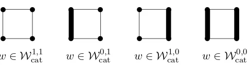
w∈ Wcat1,1 w∈ Wcat0,1 w∈ Wcat1,0 w∈ Wcat0,0

Figure 1: Effective boundaries for w_{∈ Wcat}.

Lemma 2.2 (Scaling property of renormalization transformations) One has

(i) νxλc,λw=νxc,w (ii) Fλc(λw) =λFcw

(λ, c >0, w_{∈ W}, x_∈D). (2.1)

The following simple lemma will play a crucial role in what follows.

Lemma 2.3 (Mean and covariance matrix) For all x _∈ D and i, j = 1, . . . , d, the mean

and covariances of νxc,w are given by

(i)

Z

D

ν_xc,w(dy)(yi−xi) = 0,

(ii) Z

D

ν_xc,w(dy)(yi−xi)(yj −xj) = 1_cFcwij(x).

(2.2)

For anyw∈ C(D, M₊d), we call

∂wD:={x∈D:wij(x) = 0 ∀i, j= 1, . . . , d} (2.3)

the effective boundary of D (associated with w). If y is a solution to the martingale problem

for the operator Pd

i,j=1wij(y) ∂ 2

∂yi∂yj (i.e., the operator in (1.1) without the drift), then, by

martingale convergence, yt converges a.s. to a limit y∞; it is not hard to see that y∞ ∈∂wD a.s. The next lemma says that the effective boundary is invariant under renormalization.

Lemma 2.4 (Invariance of effective boundary) One has ∂FcwD = ∂wD for all w ∈ W,

c >0.

For example, for diffusion matrices w from the renormalization class W = Wcat, there oc-cur four different effective boundaries, depending on whether w _{∈ W}_cat1,1, _W_cat0,1, _W_cat1,0, or _W_cat0,0. These effective boundaries are depicted in Figure1. The statement from Theorem1.4 (a) that Fc(Wcatl,r)⊂ Wcatl,r is just the translation of Lemma 2.4to the special set-up there.

(9)

probability kernelsKw,(n) associated with a diffusion matrixw∈ W (and the constants (ck)k≥0) are the probability kernels onD defined inductively by

K_xw,(n+1)(dz) := Z

D

νcn,F(n)w

x (dy)Kyw,(n)(dz) (n≥0) with Kxw,(0)(dy) :=δx(dy), (2.4)

withF(n) as in (1.8). Note that

F(n)w(x) = Z

D

K_xw,(n)(dy)w(y) (x_∈D, n_≥0). (2.5)

The next lemma follows by iteration from Lemmas2.1and2.3. In their essence, this lemma and Lemma2.6 below go back to [BCGdH95].

Lemma 2.5 (Basic properties of iterated probability kernels) For each w _{∈ W}, the

Kw,(n) _{are continuous probability kernels on} _D_{. Moreover, for all} _x _∈ _D_, _{i, j} _{= 1, . . . , d}_{, and}

n≥0, the mean and covariance matrix of Kxw,(n) are given by

(i)

Z

D

K_xw,(n)(dy)(yi−xi) = 0,

(ii) Z

D

K_xw,(n)(dy)(yi−xi)(yj−xj) =snF(n)wij(x).

(2.6)

We equip the space _C(D,_M1(D)) of continuous probability kernels on D with the topology of uniform convergence (since _M1(D) is compact, there is a unique uniform structure on _M1(D) generating the topology). For ‘nice’ renormalization classes, it seems reasonable to conjecture that the kernelsKw,(n)converge asn_{→ ∞}to some limitKw,∗ in_C(D,_M1(D)). If this happens, then formula (2.6) (ii) tells us that the rescaled renormalized diffusion matricessnF(n)wconverge uniformly on D to the covariance matrix of Kw,∗. This gives a heuristic explanation why we need to rescale the iterates F(n)w with the scaling constants sn from (1.9) to get a nontrivial limit in (1.11).

We now explain the relevance of the conditions (1.10) (i) and (ii) in the present more general context. If the iterated kernels converge to a limit Kw,∗, then condition (1.10) (i) guarantees that this limit is concentrated on the effective boundary:

Lemma 2.6 (Concentration on the effective boundary) If sn −→

n→∞ ∞, then for any f ∈

C(D) such that f = 0 on ∂wD:

lim n→∞sup

x∈D Z

D

K_xw,(n)(dy)f(y)

= 0. (2.7)

In fact, the condition sn → ∞ guarantees that the corresponding system of hierarchically in-teracting diffusions with migration constants (ck)k≥0 clusters in the local mean field limit, see [DG93a, Theorem 3] or AppendixA.1 below.

(10)

For this purpose, it will be convenient to modify the definition of our scaling constantssna little bit. Fix someβ >0 and put

sn:=β+sn (n≥0). (2.8)

Define rescaled renormalization transformationsFγ :W → W by

Fγw:= (1 +γ)F1/γw (γ >0, w ∈ W). (2.9)

Using (2.1) (ii), one easily deduces that

snF(n)w=Fγn−1◦ · · · ◦Fγ0(βw) (w∈ W, n≥1), (2.10)

where

γn:= 1

sncn (n≥0). (2.11)

We can reformulate the conditions (1.10) (i) and (ii) in terms of the constants (γn)n≥0. Indeed, it is not hard to check1 _{that equivalent formulations of condition (}_1.10_{) (i) are:}

(i) sn_n→∞−→ ∞, (ii) sn_n→∞−→ ∞, (iii) X n

γn=∞. (2.12)

Since sn+1/sn = 1 +γn we see moreover that, for any γ∗ ∈ [0,∞], equivalent formulations of condition (1.10) (ii) are:

(i) sn+1 sn n→∞−→

1 +γ∗, (ii) sn+1 sn n→∞−→

1 +γ∗, (iii) γn_n→∞−→ γ∗. (2.13)

If 0< γ∗ <∞, then, in the light of (2.10), we expectsnF(n)wto converge to a fixed point of the transformationFγ∗. Ifγ∗ = 0, the situation is more complex. In this case, we expect the orbit

snF(n)w7→sn+1F(n+1)w7→ · · ·, for large n, to approximate a continuous flow, the generator of which is

lim γ→0γ

−1_F_γw₋_w_{(x) =} 1 2

d X

i,j=1

wij(x)_∂x∂2

i∂xjw(x) +w(x) (x∈D). (2.14)

To see that the right-hand side of this equation equals the left-hand side if w is twice contin-uously differentiable, one needs a Taylor expansion of w together with the moment formulas (2.2) forνx1/γ,w. Under condition condition (2.12) (iii), we expect this continuous flow to reach equilibrium.

In the light if these considerations, we are led to at the following general conjecture.

Conjecture 2.7 (Limits of rescaled renormalized diffusion matrices)Assume thatsn→

∞ and sn+1/sn→1 +γ∗ for some γ∗∈[0,∞]. Then, for anyw∈ W,

∗_, _(2.15)

1_{To see this, let} _s

∞ ∈ (0,∞] denote the limit of the sn and note that on the one hand, P_n1/(sncn) ≥

P

nlog(1 + 1/(sncn)) = log(Qnsn+1/sn) = log(s∞/s1), while on the other hand Pn1/(sncn) ≤ Qn(1 +

(11)

where w∗ satisfies

(i) Fγ∗w∗=w∗ if 0< γ∗ <∞,

(ii) 1₂ d X

i,j=1

w∗_ij(x)_∂x∂2

i∂xjw

∗_{(x) +}_w∗_{(x) = 0} _(x

∈D) if γ∗ = 0,

(iii) lim

γ→∞Fγw

∗₌_w∗ _if _γ∗ ₌_∞_.

(2.16)

We call (2.16) (ii), which is in some sense theγ∗→0 limit of the fixed point equation (2.16) (i),

the asymptotic fixed point equation. A version of formula (2.16) (ii) occured in [Swa99,

for-mula (1.3.5)] (a minus sign is missing there).

In particular, one may hope that for a given effective boundary, the equations in (2.16) have a unique solution. Our main result (Theorem1.4) confirms this conjecture for the renormalization class Wcat and for γ∗ < ∞. In the next section, we discuss numerical evidence that supports Conjecture2.7in the case γ∗= 0 for other renormalization classes on compacta as well.

In previous work on renormalization classes, fixed shapes have played an important role. By definition, for any prerenormalization class _W, a fixed shapeis a subclass ˆ_{W ⊂ W} of the form

ˆ

W = {λw : λ > 0} with 0 6= w ∈ W, such that Fc( ˆW) ⊂ Wˆ for all c > 0. The next lemma describes how fixed shapes for renormalization classes on compact sets typically arise.

Lemma 2.8 (Fixed shapes)Assume that for each0< γ∗ _<_∞_{, there is a}₀₆₌_w∗₌_w∗ γ∗ ∈ W

such thatsnF(n)w −→

n→∞w ∗

γ∗ whenever w∈ W, s_n→ ∞, ands_n+1/s_n→1 +γ∗. Then:

(a)w_γ∗∗ is the unique solution in W of equation (2.16) (i).

(b) If w∗ =w∗_γ∗ does not depend onγ∗, then

Fc(λw∗) = (_λ1 +1_c)−1w∗ (λ, c >0). (2.17)

Moreover, _{λw∗:λ >0_} is the unique fixed shape in _W.

(c)If thew_γ∗∗ for different values ofγ∗ are not constant multiples of each other, thenW contains

no fixed shapes.

Note that by Theorem1.4,Wcat0,1 is a renormalization class satisfying the general assumptions of Lemma2.8. The unique solution of (2.16) (i) inWcat0,1is of the formw∗=w1,p

∗

wherep∗ =p∗_0,1,γ∗.

We conjecture that thep∗_0,1,γ∗ for different values ofγ∗ are not constant multiples of each other,

and, as a consequence, that_W_cat0,1 contains no fixed shapes.

(12)

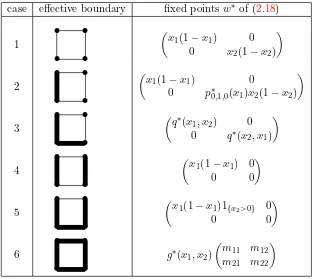
2.2 Numerical solutions to the asymptotic fixed point equation

Let t_7→ w(t, _·) be a solution to the continuous flow with the generator in (2.14), i.e., w is an M₊d-valued solution to the nonlinear partial differential equation

∂

∂tw(t, x) = 12 d X

i,j=1

wij(t, x)_∂x∂2

i∂xjw(t, x) +w(t, x) (t≥0, x∈D). (2.18)

Solutions to (2.18) are quite easy to simulate on a computer. We have simulated solutions for all kind of diffusion matrices (including nondiagonal ones) on the unit square [0,1]2, with the effective boundaries 1–6 depicted in Figure2. For all initial diffusion matricesw(0,_·) we tried, the solution converged ast→ ∞to a fixed pointw∗. In all cases except case 6, the fixed point was unique. The fixed points are listed in Figure 2. The functions p∗_0,1,0 and q∗ from Figure 2

are plotted in Figure3. Here p∗_0,1,0 is the function from Theorem 1.4(c).

The fixed points for the effective boundaries in cases 1,2, and 4 are the unique solutions of equation (1.12) (ii) from Theorem 1.4 in the classes Wcat1,1, Wcat0,1, and Wcat0,0, respectively. The simulations suggest that the domain of attraction of these fixed points (within the class of “all” diffusion matrices on [0,1]2_{) is actually a lot larger than the classes}_W1,1

cat,Wcat0,1, and Wcat0,0. The functionq∗ from case 3 satisfiesq∗(x1,1) =x1(1−x1) and is zero on the other parts of the boundary. In contrast to what one might perhaps guess in view of case 2,q∗ isnot of the form q∗_(x

1, x2) =f(x2)x1(1−x1) for some function f.

Case 5 is somewhat degenerate since in this case the fixed point is not continuous.

The only case where the fixed point is not unique is case 6. Here, m can be any positive definite matrix, while g∗, depending on m, is the unique solution on (0,1)2 of the equation 1 +1₂P2

i,j=1mij ∂ 2 ∂xi∂xig

∗_{(x) = 0, with zero boundary conditions.}

2.3 Previous rigorous results

In this section we discuss some results that have been derived previously for renormalization classes on compact sets.

Theorem 2.9 [BCGdH95, DGV95] (Universality class of Wright-Fisher models) Let

D := _{x _∈ Rd _: _x_i _> ₀ _∀_i, Pd

i=1xi < 1}, and let {e0, . . . , ed}, with e0 := (0, . . . ,0) and

e1 := (1,0, . . . ,0), . . . , ed:= (0, . . . ,0,1)be the extremal points of D. Let wij∗(x) :=xi(δij −xj) (x_∈D,i, j= 1, . . . , d)denote the standard Wright-Fisher diffusion matrix, and assume that _W

is a renormalization class on D such that w∗ ∈ W and ∂wD={e0, . . . , ed} for all w∈ W. Let

(ck)k≥0 be migration constants such that sn → ∞ as n → ∞. Then, for all w∈ W, uniformly

onD,

snF(n)w_n→∞−→ w∗. (2.19)

(13)

case effective boundary fixed points w∗ of (2.18)

Figure 2: Fixed points of the flow (2.18).

(14)

of finding a nontrivial example of such a renormalization class is open in dimensions greater than one. In the one-dimensional case, however, the following result is known.

Lemma 2.10 [DG93b] (Renormalization class on the unit interval) The set

WDG:={w∈ C[0,1] :w= 0 on{0,1}, w >0 on (0,1), w Lipschitz} (2.20)

is a renormalization class on [0,1].

About renormalization of isotropic diffusions, the following result is known. Below,∂D:=D\D denotes the topological boundary ofD.

Theorem 2.11 [dHS98] (Universality class of isotropic models) Let D _⊂ Rd _{be open,}

bounded, and convex and let m _∈ Md

+ be fixed and (strictly) positive definite. Set w∗ij(x) :=

mijg∗(x), where g∗ is the unique solution of 1 + 1₂Pijmij ∂

2 ∂xi∂xjg

∗_{(x) = 0} _for _x _∈ _D _and g∗_{(x) = 0} _for _x_∈_∂D_{. Assume that} _W _{is a renormalization class on} _D _{such that} _w∗ _{∈ W} _and

such that each w∈ W is of the form

wij(x) =mijg(x) (x∈D, i, j= 1, . . . , d), (2.21)

for some g_{∈ C}(D) satisfying g >0 on D and g= 0 on∂D. Let (ck)k≥0 be migration constants

such thatsn→ ∞ as n→ ∞. Then, for allw∈ W, uniformly on D,

∗_. _(2.22)

The proof of Theorem 2.11 follows the same lines as the proof of Theorem 2.9, with the dif-ference that in this case one needs to generalize the first moment formula (2.6) (i) in the sense that R

DK w,(n)

x (dy)h(y) = h(x) for any m-harmonic function h, i.e., h ∈ C(D) satisfy-ing P

ijmij ∂ 2

∂xi∂xjh(x) = 0 for x ∈ D. The kernel K

w,(n)

x now converges to the m-harmonic measure on∂D with mean x, and this implies (2.22).

Again, in dimensions d ≥ 2, the problem of finding a ‘reasonable’ class W satisfying the as-sumptions of Theorem2.11is so far unresolved. The problem with verifying conditions (i)–(iv) from Definition1.1 in an explicit set-up is that (i) and (ii) usually require some smoothness of w, while (iv) requires that one can prove the same smoothness forFcw, which is difficult. The proofs of Theorems 2.9 and 2.11 are based on the same principle. For any diffusion ma-trix w, let Hw denote the class of w-harmonic functions, i.e., functions h ∈ C(D) satisfying P

ijwij(x) ∂ 2

∂xi∂xjh(x) = 0 on D. If w belongs to one of the renormalization classes in

Theo-rems 2.9 and 2.11, then Hw has the property that Tx,tc h(Hw) ⊂ Hw for all c > 0, x ∈ D, and t≥0, whereT_x,tc h(y) :=h(x+ (y−x)e−ct) is the semigroup with generator Pd

i=1c(xi−yi)_∂y∂_i, i.e., the operator in (1.1) without the diffusion part. In this case we say that w has

invari-ant harmonics; see [Swa00]. As a consequence, one can prove that the iterated kernels satisfy

R DK

w,(n)

x (dy)h(y) =h(x) for all h∈Hw and x∈D. Ifsn → ∞, then this implies that Kxw,(n) converges to the unique Hw-harmonic measure on ∂wD with mean x. Diffusion matrices from Wcatdo not in general have invariant harmonics. Therefore, to prove Theorem1.4, we need new techniques.

(15)

3 Connection with branching theory

From now on, we focuss on the renormalization class _Wcat. We will show that for this renor-malization class, the rescaled renorrenor-malization transformationsFγ from (2.9) can be expressed in terms of the log-Laplace operators of a discrete time branching process on [0,1]. This will allow us to use techniques from the theory of spatial branching processes to verify Conjecture2.7 for the renormalization class Wcat in the case γ∗ <∞.

3.1 Poisson-cluster branching processes

We first need some concepts and facts from branching theory. Finite measure-valued branching processes (on R) in discrete time have been introduced by Jiˇrina [Jir64]. We need to consider only a special class. Let E be a separable, locally compact, and metrizable space. We call a continuous map _Q fromE into _M1(_M(E)) acontinuous cluster mechanism. By definition, an M(E)-valued random variable_X is a Poisson cluster measureonE with locally finiteintensity

measure µand continuous cluster mechanism Q, if its log-Laplace transform satisfies

−logE

e−hX, fi=

Z

E

µ(dx)1− Z

M(E)Q

(x,dχ)e−hχ, fi

(f ∈B+(E)). (3.1)

For givenµandQ, such a Poisson cluster measure exists, and is unique in distribution, provided that the right-hand side of (3.1) is finite forf = 1. It may be constructed as_X =P

iχxi, where

P

iδxi is a (possibly infinite) Poisson point measure with intensity µ, and givenx1, x2, . . ., the

χx1, χx2, . . . are independent random variables with lawsQ(x1,·),Q(x2,·), . . ., respectively. Now fix a finite sequence of functions qk ∈ C+(E) and continuous cluster mechanismsQk (k= 1, . . . , n), define

Ukf(x) :=qk(x)

1− Z

M(E)Qk

(x,dχ)e−hχ, fi

(x∈E, f ∈B+(E), k = 1, . . . , n), (3.2)

and assume that

sup x∈EUk

1(x)<_∞ (k= 1, . . . , n). (3.3)

Then _Uk maps B+(E) intoB+(E) for each k, and for eachM(E)-valued initial state X0, there exists a (time-inhomogeneous) Markov chain (X0, . . . ,Xn) inM(E), such that Xk, givenXk−1, is a Poisson cluster measure with intensity qkXk−1 and cluster mechanism Qk. It is not hard to see that

Eµ

e−hXn, fi=e−hµ,U1◦ · · · ◦ Unfi (µ∈ M(E), f ∈B+(E)). (3.4)

We call _X = (_X0, . . . ,_Xn) the Poisson-cluster branching process on E with weight functions

q1, . . . , qnand cluster mechanismsQ1, . . . ,Qn. The operatorUkis called thelog-Laplace operator of the transition law fromXk−1 toXk. Note that we can write (3.4) in the suggestive form

Pµ

Pois(f_Xn) = 0 =P

Pois (_U1_{◦ · · · ◦ Un}f)µ = 0

. (3.5)

(16)

3.2 The renormalization branching process

We will now construct a Poisson-cluster branching process on [0,1] of a special kind, and show that the rescaled renormalization transformations on _Wcat can be expressed in terms of the log-Laplace operators of this branching process.

By Corollary5.4below, for each γ >0 andx∈[0,1], the SDE

dy(t) = 1_γ(x₋y(t))dt+p2y(t)(1₋y(t))dB(t), (3.6)

has a unique (in law) stationary solution. We denote this solution by (yxγ(t))t∈R. Let τγ be an independent exponentially distributed random variable with mean γ, and define a random measure on [0,1] by

Zxγ := Z τγ

0 δ_yγ

x(−t/2)dt (γ >0, x∈[0,1]). (3.7)

The Poisson-cluster branching process that we are about to define will have clusters that are distributed as_Zxγ. To define its (constant) weight functions and its continuous (by Corollary5.10 below) cluster mechanisms, we put

qγ:= 1_γ + 1 and Qγ(x,·) :=L(Zxγ) (γ >0, x∈[0,1]). (3.8)

We let_Uγ denote the log-Laplace operator with weight function qγ and cluster mechanismQγ, i.e.,

Uγf(x) :=qγ1− Z

M([0,1])Qγ(x,

dχ)e−hχ, fi

(x∈[0,1], f ∈B+[0,1], γ >0). (3.9)

We now establish the connection between renormalization transformations on Wcat and log-Laplace operators.

Proposition 3.1 (Identification of the renormalization transformation) Let Fγ be the

rescaled renormalization transformation on Wcat defined in (2.9). Then

Fγw1, p=w1,Uγp (p∈ H, γ >0). (3.10)

Fix a diffusion matrixwα,p_{∈ Wcat}_{and migration constants (c}

k)k≥0. Define constantssnandγn as in (2.8) and (2.11), respectively, where β := 1/α. Then Proposition 3.1 and formula (2.10) show that

snF(n)wα,p =w1,Uγn−1◦ · · · ◦ Uγ0( p

α). (3.11)

(17)

3.3 Convergence to a time-homogeneous process

LetX = (X−n, . . . ,X0) be the renormalization branching process introduced in the last section. If the constants (γk)k≥0 satisfyPnγn=∞andγn→γ∗ for someγ∗∈[0,∞), thenX is almost time-homogeneous for largen. More precisely, we will prove the following convergence result.

Theorem 3.2 (Convergence to a time-homogenous branching process) Assume that

L(_X−n) =⇒

is the time-homogenous branching process with log-Laplace operatorUγ∗ in each step

and initial law _L(_Y₀γ∗) =µ.

l=k γl ≤ t}, and Y0 is the super-Wright-Fisher diffusion with activity and growth

parame-ter both identically 1 and initial law _L(_Y₀0) =µ.

The super-Wright-Fisher diffusion was studied in [FS03]. By definition,_Y0 _{is the} time-homoge-neous Markov process in M[0,1] with continuous sample paths, whose Laplace functionals are given by

tf =ut is the unique mild solution of the semilinear Cauchy equation (

For a further study of the renormalization branching process _X and its limiting processes _Yγ∗

(γ∗ ≥0) we will use the technique of embedded particle systems, which we explain in the next section.

3.4 Weighted and Poissonized branching processes

In this section, we explain how from a Poisson-cluster branching process it is possible to construct other branching processes by weighting and Poissonization. We first need to introduce spatial branching particle systems in some generality.

(18)

We call a continuous map x 7→Q(x,·) from E into M1(N(E)) a continuous offspring mecha-nism.

Fix continuous offspring mechanisms Qk (1≤k≤n), and let (X0, . . . , Xn) be a Markov chain in _N(E) such that, given that Xk−1 = Pmi=1δxi, the next step of the chain Xk is a sum of

independent random variables with laws Qk(xi,·) (i= 1, . . . , m). Then

Eν

(1−f)Xn

= (1−U1◦ · · · ◦Unf)ν (ν ∈ N(E), f ∈B[0,1](E)), (3.17)

whereUk :B[0,1](E)→B[0,1](E) is defined as

Ukf(x) := 1− Z

N(E)

Qk(x,dν)(1−f)ν (1≤k≤n, x∈E, f ∈B[0,1](E)). (3.18)

We call Uk the generating operator of the transition law from Xk−1 to Xk, and we call X = (X0, . . . , Xn) the branching particle system on E with generating operators U1, . . . , Un. It is often useful to write (3.17) in the suggestive form

Pν

Thinf(Xn) = 0

=P

ThinU1◦···◦Unf(ν) = 0

(ν ∈ N(E), f ∈B[0,1](E)). (3.19)

Here, if ν is an N(E)-valued random variable and f ∈ B[0,1](E), then Thinf(ν) denotes an N(E)-valued random variable such that conditioned on ν, Thinf(ν) is obtained from ν by independently throwing away particles from ν, where a particle at x is kept with probability f(x). One has the elementary relations

Thinf(Thing(ν))

D

= Thinf g(ν) and Thinf(Pois(µ))

D

= Pois(f µ), (3.20)

where= denotes equality in distribution.D

We are now ready to describe weighted and Poissonized branching processes. Let _X = (X0, . . . ,Xn) be a Poisson-cluster branching process on E, with continuous weight functions q1, . . . , qn, continuous cluster mechanisms Q1, . . . ,Qn, and log-Laplace operators U1, . . . ,Un given by (3.2) and satisfying (3.3). Let _Zk

x denote an M(E)-valued random variable with law Qk(x, ·). Let h ∈ C+(E) be bounded, h 6= 0, and put Eh := {x ∈ E : h(x) > 0}. For f ∈B+(Eh), define hf ∈B+(E) by hf(x) :=h(x)f(x) ifx∈Eh and hf(x) := 0 otherwise.

Proposition 3.3 (Weighting of Poisson-cluster branching processes)Assume that there

exists a constantK <_∞ such that _Ukh_≤Kh for all k= 1, . . . , n. Then there exists a

Poisson-cluster branching process _Xh _{= (}_Xh

0, . . . ,Xnh) onEh with weight functions(qh1, . . . , qnh) given by

q_kh:=qk/h, continuous cluster mechanisms Qh1, . . . ,Qhn given by

Qkh(x,·) :=L(hZxk) (x∈Eh), (3.21)

and log-Laplace operatorsUh

1, . . . ,Unh satisfying

hUkhf :=Uk(hf) (f ∈B+(Eh)). (3.22)

The processes X andXh are related by

(19)

Proposition 3.4 (Poissonization of Poisson-cluster branching processes) Assume that

Ukh≤h for all k= 1, . . . , n. Then there exists a branching particle system Xh = (X₀h, . . . , X_nh)

onEh _{with continuous offspring mechanisms} _Qh

1, . . . , Qhn given by

Qh_k(x,·) := qk(x) h(x)P

Pois(hZxk)∈ ·

+1−qk(x) h(x)

δ0(·) (x∈Eh), (3.24)

and generating operators Uh

1, . . . , Unh satisfying

hU_khf :=_Uk(hf) (f _∈B_[0,1](Eh)). (3.25)

The processes X andXh are related by

L(X₀h) =_L(Pois(h_X0)) implies _L(X_kh) =_L(Pois(h_Xk)) (0_≤k_≤n). (3.26)

Here, the right-hand side of (3.24) is always a probability measure, despite that it may happen that qk(x)/h(x) > 1. The (straightforward) proofs of Propositions 3.3 and 3.4 can be found in Section 7.1 below. If (3.23) holds then we say that Xh _{is obtained from} _X _by _weighting with density h. If (3.26) holds then we say thatXh _{is obtained from}_X _by _{Poissonization}_with density h. Proposition 3.4 says that a Poisson-cluster branching process X contains, in a way, certain ‘embedded’ branching particle systems Xh. Poissonization relations for superprocesses and embedded particle systems have enjoyed considerable attention, see [FS04] and references therein.

A functionh _∈B+(E) such that Ukh ≤h is called Uk-superharmonic. If the reverse inequality holds we say thath is Uk-subharmonic. If Ukh=h thenh is called Uk-harmonic.

3.5 Extinction versus unbounded growth for embedded particle systems

In this section we explain how embedded particle systems can be used to prove Theorem 1.4. Throughout this section (γk)k≥0 are positive constants such that Pnγn =∞ and γn →γ∗ for some γ∗ _∈ [0,_∞), and _X = (_X−n, . . . ,_X0) is the renormalization branching process on [0,1] defined in Section3.2. We write

U(n) :=_Uγ_n₋₁_{◦ · · · ◦ Uγ}₀. (3.27)

In view of formula (3.11), in order to prove Theorem1.4, we need the following result.

Proposition 3.5 (Limits of iterated log-Laplace operators) Uniformly on[0,1],

(i) lim n→∞U

(n)_p_{= 1} _(p_{∈ H1,1}_),

(ii) lim n→∞U

(n)_p_{= 0} _(p_{∈ H0,0}_),

(iii) lim n→∞U

(n)_p₌_p∗

0,1,γ∗ (p∈ H0,1),

(3.28)

(20)

In our proof of Proposition 3.5, we will use embedded particle systems Xh = (X_−nh , . . . , X₀h) obtained fromX by Poissonization with functionsh1,1,h0,0andh0,1 taken from the classesH1,1, H0,0, and_H0,1, respectively. More precisely, we will use the functions

h1,1(x) := 1,

The choice of these functions is up to a certain degree arbitrary, and guided by what is most convenient in proofs. This applies in particular to the function h0,1; see the remarks following Lemma3.8.

Lemma 3.6 (Embedded particle system with h1,1) The function h1,1 from (3.29) is Uγ

-harmonic for each γ >0. The corresponding embedded particle system Xh1,1 _on_[0,_1]_satisfies

P−n,δx

In (3.30) and similar formulas below, _⇒ denotes weak convergence of probability measures on [0,_∞]. Thus, (3.30) says that for processes started with one particle on the positionx at times −n, the number of particles at time zero converges to infinity as n→ ∞.

-superharmonic for each γ > 0. The corresponding embedded particle system Xh0,0 _on _(0,₁₎ _is

critical and satisfies

Here, a branching particle system X is called critical if each particle produces on average one offspring (in each time step and independent of its position). Formula (3.31) says that the em-bedded particle systemXh0,0 _{gets extinct during the time interval}_{−_{n, . . . ,}₀_}_{with probability} tending to one asn_{→ ∞}. We can summarize Lemmas3.6and3.7by saying that the embedded particle system associated with h1,1 grows unboundedly while the embedded particle system associated withh0,0 becomes extinct asn→ ∞.

We now consider the embedded particle system Xh0,1 _with _h

0,1 ∈ H0,1 as in (3.29). It turns out that this system either gets extinct or grows unboundedly, each with a positive probability. In order to determine these probabilities, we need to consider embedded particle systems for the time-homogeneous processes _Yγ∗

(γ∗ _∈[0,_∞)) from (3.12) and (3.13). If h _{∈ H0,1} is _Uγ∗

-superharmonic for some γ∗ > 0, then Poissonizing the process Yγ∗

with h yields a branching

1[0,∞] is compact in the topology of weak convergence, there is a unique uniform structure compatible with the topology, and therefore it makes sense to talk about uniform convergence ofM1[0,∞]-valued functions (in this case,x7→P−n,δxˆ|Xh1,1

0 | ∈ · ˜

(21)

then Poissonizing the super-Wright-Fisher diffusionY0_with_h_{yields a continuous-time branching} particle system on (0,1], which we denote by Y0,h = (Y_t0,h)t≥0. For example, for m ≥ 4, the functionh(x) := 1₋(1₋x)m _{satisfies (}_3.32_).

-superharmonic for each γ > 0. The corresponding embedded particle system Xh0,1 _on _(0,_1]

satisfies

P−n,δx |Xh0,1

0 | ∈ ·

=_⇒

n→∞ργ∗(x)δ∞+ (1−ργ∗(x))δ0, (3.33)

locally uniformly for all x∈(0,1], where

ργ∗(x) :=

(

Pδx_[Yγ∗,h0,1

k 6= 0 ∀k≥0] (0< γ∗ <∞), Pδx_[Y0,h0,1

t 6= 0 ∀t≥0] (γ∗ = 0).

(3.34)

Lemma3.8is one of the most technical lemmas in this paper. In all places where it is used,h0,1 could be replaced by any other function with roughly the same shape (concave, increasing, with finite slope at zero) that isUγ-superharmonic for eachγ >0. The problem is to show that such functions exist at all. Functions of the formh(x) := 1₋(1₋x)m are convenient in calculations, since they can be treated using duality. The lowest value of the exponent for which our bounds work turns out to bem= 7.

We now explain how Lemmas 3.6–3.8 imply Proposition 3.5. In doing so, it will be more con-venient to work with weighted branching processes than with Poissonized branching processes. A little argument (which can be found in Lemma7.12 below) shows that Lemmas 3.6–3.8 are equivalent to the next proposition.

Proposition 3.9 (Extinction versus unbounded growth)Let h1,1, h0,0, and h0,1 be as in

(3.29). Forγ∗_∈[0,_∞), put p_1,1,γ∗ ∗(x) := 1, p∗_0,0,γ∗(x) := 0 (x∈[0,1]), and

p∗_0,1,γ∗(0) := 0 and p∗_0,1,γ∗(x) :=h_0,1(x)ρ_γ∗(x) (x∈(0,1]), (3.35)

withργ∗ as in (3.34). Then, for (l, r) = (1,1),(0,0), and(0,1),

P−n,δx

hX0, hl,ri ∈ · =⇒ n→∞e

−p∗_l,r,γ∗(x)

δ0+ 1−e−p

∗

l,r,γ∗(x)

δ∞, (3.36)

uniformly for all x_∈[0,1].

Formula (3.36) says that the weighted branching process _Xhl,r _{exhibits a form of ‘extinction}

versus unbounded growth’. More precisely, for large n the total mass of hl,rX0 is close to 0 or ∞ with high probability.

Proof of Proposition 3.5By (3.4),

U(n)p(x) =₋logE−n,δx

e−hX0, pi (p∈B₊[0,1], x∈[0,1]). (3.37)

We first prove formula (3.28) (ii). For (l, r) = (0,0), formula (3.36) says that

P−n,δx_[_hX0_{, h}_{0,0i ∈ ·}_{] =}_⇒

(22)

uniformly for all x∈[0,1]. If p∈ H0,0, then we can findr >0 such that p≤rh0,0. Therefore,

Using moreover (3.38), we see that

P−n,δx_[_hX0_{, p}_{i ∈ ·}_{] =}_⇒

ξ∈Z2 is a collection of independent Brownian motions. We call x a system of linearly interacting catalytic Wright-Fisher diffusions with catalyzation functionp. It is expected thatx

clusters, i.e.,x(t) converges in distribution ast_{→ ∞} to a limit (xξ(∞))ξ∈Z2 such thatx_ξ(∞) =

(23)

solution of the asymptotic fixed point equation (2.16) (ii) in the renormalization classWcat0,1; see ConjectureA.3in AppendixA.2 below.

The present paper is inspired by the work of Greven, Klenke and Wakolbinger [GKW01]. They study a model that is closely related to (4.1), but where x1 _{is replaced by a voter model. They} show that their model clusters and determine its clustering distribution_L(x0(∞)), which turns out to coincide with the mentioned prediction for (4.1) based on renormalization theory. In fact, they believe their results to hold for the model in (4.1) too, but they could not prove this due to certain technical difficulties that a [0,1]-valued catalyst would create, compared to the simpler {0,1}-valued voter model.

The work in [GKW01] not only provides the main motivation for the present paper, but also inspired some of our techniques for proving Theorem 1.4. This concerns in particular the proof of Proposition3.1, which makes the connection between renormalization transformations and a branching process. We hope that conversely, our techniques may shed some light on the problems left open by [GKW01], in particular, the question whether their results stay true if the voter model catalyst is replaced by a Wright-Fisher catalyst. It seems plausible that their results may not hold for the model in (4.1) if the catalyzing function p grows too fast at 0. On the other hand, our proofs suggest that p with a finite slope at 0 should be OK. (In particular, while deriving formula (3.41), we use that p can be bounded from above byr+h0,1 for some r+>0, which requires that phas a finite slope at 0.)

Our results are also interesting in the wider program of studying renormalization classes in the sense of Definition 1.1. We conjecture that the class _W_cat0,1, unlike all renormalization classes studied previously, contains no fixed shapes (see the discussion following Lemma2.8). In fact, we expect this to be the usual situation. In this sense, the renormalization classes studied so far were all of a special type.

4.2 Open problems

(24)

Even for the renormalization classWcat, several interesting problems are left open. One of the most urgent ones is to prove that the functionsp∗_0,1,γ∗ are not constant in γ∗, and therefore, by

Lemma2.8 (c),Wcat0,1 contains no fixed shapes. Moreover, we have not investigated the iterated renormalization transformations in the regime γ∗ = _∞. Also, we believe that the convergence in (3.28) (ii) does not hold if the condition that pis Lipschitz is dropped, in particular, if phas an infinite slope at 0 or an infinite negative slope at 1. For p∈ H0,0, it seems plausible that a properly rescaled version of the iterates _U(n)p converges to a universal limit, but we have not investigated this either. Finally, we have not investigated the convergence of the iterated kernels Kw,(n) from (2.4) (in particular, we have not verified Conjecture A.2) for the renormalization class_Wcat.

Our methods, combined with those in [BCGdH95], can probably be extended to study the action of iterated renormalization transformations on diffusion matrices of the following more general form (compared to (1.4)):

w(x) =

g(x1) 0

0 p(x1)x2(1−x2)

(x=_∈[0,1]2), (4.2)

where g : [0,1] _→ R is Lipschitz, g(0) = g(1) = 0, g > 0 on (0,1), and p _{∈ H} as before. This would, however, require a lot of extra technical work and probably not generate much new insight. The numerical simulations mentioned in Section 2.2 suggest that many diffusion matrices of an even more general form than (4.2) also converge under renormalization to the limit pointsw∗ from Theorem1.4, but we don’t know how to prove this.

Part II

Outline of Part IIIn Section5, we verify that_Wcatis a renormalization class, we prove Propo-sition 3.1, which connects the renormalization transformations Fc to the log-Laplace operators Uγ, and we collect a number of technical properties of the operatorsUγ that will be needed later on. In Section6we prove Theorem 3.2about the convergence of the renormalization branching process to a time-homogeneous limit. In Section 7, we prove the statements from Section 3.5

about extinction versus unbounded growth of embedded particle systems, with the exception of Lemma 3.7, which is proved in Section 8. In Section 9, finally, we combine the results derived by that point to prove our main theorem.

5 The renormalization class

_W

_cat

(25)

5.1 Renormalization classes on compact sets

In this section, we prove the lemmas stated in Section2. Recall thatD_⊂Rd_{is open, bounded,}

and convex, and that W is a prerenormalization class on D, equipped with the topology of uniform convergence.

Proof of Lemma 2.1To see that (x, c, w)7→νxc,w is continuous, let (xn, cn, wn) be a sequence converging in D_×(0,_∞) _{× W} to a limit (x, c, w). By the compactness of D, the sequence (νcn,wn

xn )n≥0 is tight, and each limit point ν∗ satisfies

hν∗, Ac,w_x f_i= 0 (f _{∈ C}(2)(D)). (5.1) Therefore, by [EK86, Theorem 4.9.17],ν∗ _{is an invariant law for the martingale problem} associ-ated withAc,wx . Since we are assuming uniqueness of the invariant law,ν∗=νxc,w and therefore νcn,wn

xn ⇒ν

c,w

x . The continuity ofFcw(x) is a simple consequence of the continuity of νxc,w.

Proof of Lemma2.2Formula (2.1) (i) follows from the fact that rescaling the time in solutions (yt)t≥0 to the martingale problem for Ac,wx by a factor λhas no influence on the invariant law. Formula (2.1) (ii) is a direct consequence of formula (2.1) (i).

Proof of Lemma 2.3 This follows by inserting the functions f(x) = xi and f(x) =xixj into the equilibrium equation (5.1).

Proof of Lemma 2.4 If x ∈ ∂wD, then yt := x (t ≥ 0) is a stationary solution to the

martingale problem for Ac,wx , and therefore νxc,w = δx and Fcw(x) = w(x) = 0. On the other hand, ifx _6∈ ∂wD, then yt :=x (t≥ 0) is not a stationary solution to the martingale problem for Ac,wx and therefore R_Dνxc,w(dy)|y−x|2 > 0. Let tr(w(y)) := P_iwii(y) denote the trace of w(y). By (2.2) (ii), 1_ctr(Fcw)(x) =1_c

R Dν

c,w

x (dy)tr(w(y)) =R_Dνxc,w(dy)|y−x|2>0 and therefore Fcw(x)6= 0.

From now on assume that_W is a renormalization class. Note that

Kw,(n)=νcn−1,F(n−1)w_{· · ·}_νc0,w _(n_≥_1), _(5.2) where we denote the composition of two probability kernelsK, Lon Dby

(KL)x(dz) := Z

D

Kx(dy)Ly(dz). (5.3)

Proof of Lemma 2.5 This is a direct consequence of Lemmas 2.1 and 2.3. In particular, the

relations (2.6) follow by iterating the relations (2.2).

Proof of Lemma 2.6 Recall that tr(w(y)) denotes the trace of w(y). Formulas (2.5) and

(2.6) (ii) show that

Z

D

K_xw,(n)(dy)_|y₋x_|2=sn Z

D

K_xw,(n)(dy) tr(w(y)). (5.4)

SinceDis compact, the left-hand side of this equation is bounded uniformly inx_∈Dandn_≥1, and therefore, since we are assumingsn→ ∞,

lim n→∞_x∈Dsup

Z

D

(26)

Since w is symmetric and nonnegative definite, tr(w(y)) is nonnegative, and zero if and only if y ∈∂wD. If f ∈ C(D) satisfies f = 0 on ∂wD, then, for every ε >0, the sets Cm := {x ∈D : |f(x)_{| ≥} ε+mtr(w(x))_} are compact with Cm ↓ ∅ asm↑ ∞, so there exists an m (depending on ε) such that|f|< ε+mtr(w). Therefore,

lim sup n→∞ _x∈Dsup

Z

D

K_xw,(n)(dy)f(y)

≤lim sup n→∞ _x∈Dsup

Z

D

K_xw,(n)(dy)|f(y)|

≤ε+mlim sup n→∞ _x∈Dsup

Z

D

K_xw,(n)(dy)tr(w(y)) =ε.

(5.6)

Since ε >0 is arbitrary, (2.7) follows.

Proof of Lemma 2.8 By (2.10), (2.12), and (2.13), w∗_γ∗ = lim_n→∞(F_γ∗)nw for each w ∈ W.

By Lemma 2.1(b), Fγ∗ :W → W is continuous, so w∗_γ∗ is the unique fixed point ofF_γ∗. This

proves part (a).

Now let 0 ₆= w _{∈ W} and assume that ˆ_W = _{λw : λ > 0_} is a fixed shape. Then ˆ_{W ∋} snF(n)w_n→∞−→ w_γ∗∗ whenever sn→ ∞ and sn+1/sn→1 +γ∗ for some 0< γ∗<∞, which shows

that ˆ_W =_{λw∗_γ∗ :λ > 0}. Thus, W can contain at most one fixed shape, and if it does, then

thew_γ∗∗ for different values of γ∗ must be constant multiples of each other. This proves part (c)

and the uniqueness statement in part (b).

To complete the proof of part (b), note that if w∗ =w_γ∗∗ does not depend on γ∗, then w∗ ∈ W

solves (2.16) (i) for all 0< γ∗ <∞, hence Fcw∗ = (1 + 1_c)−1w∗ for all c >0, and therefore, by scaling (Lemma2.2), Fc(λw∗) =λFc/λ(w∗) =λ(1 +λ_c)−1w∗ = (_λ1 +1_c)−1w∗.

5.2 Coupling of catalytic Wright-Fisher diffusions

In this section we verify condition (i) of Definition 1.1 for the class Wcat, and we prepare for the verification of conditions (ii)–(iv) in Section 5.3. In fact, we will show that the larger class _Wcat := {wα,p : α > 0, p ∈ C+[0,1]} is also a renormalization class, and the equivalents of Theorem 1.4 (a) and Proposition 3.1 remain true for this larger class. (We do not know, however, if the convergence statements in Theorem1.4(b) also hold in this larger class; see the discussion in Section 4.2.)

For eachc_≥0, w_{∈ Wcat} and x_∈[0,1]2_{, the operator} _Ac,w

x is a densely defined linear operator on _C([0,1]2_{) that maps the identity function into zero and, as one easily verifies, satisfies the} positive maximum principle. Since [0,1]2is compact, the existence of a solution to the martingale problem for Ac,wx , for each [0,1]2-valued initial condition, now follows from general theory (see [RW87], Theorem 5.23.5, or [EK86, Theorem 4.5.4 and Remark 4.5.5]).

We are therefore left with the task of verifying uniqueness of solutions to the martingale problem forAc,wx . By [EK86, Problem 4.19, Corollary 5.3.4, and Theorem 5.3.6], it suffices to show that solutions to (1.7) are pathwise unique.

Lemma 5.1 (Monotone coupling of Wright-Fisher diffusions) Assume that 0 _≤ x _≤

˜

(27)

supt≥0,ω∈ΩPt(ω)<∞. Let y,y˜ be [0,1]-valued solutions to the SDE’s

ProofThis is an easy adaptation of a technique due to Yamada and Watanabe [YW71]. Since

R Here the terms in (ii) are nonpositive, and hence, letting n _{→ ∞} and using the elementary estimate

|p

y(1−y)−p ˜

y(1−y)˜ | ≤ |y−y˜|12 (y,y˜∈[0,1]), (5.12) the properties of φn, and the fact that the processP is uniformly bounded, we find that

E[0∨(yt−y˜t)]≤E[0∨(y0−y˜0)] = 0, (5.13)

by our assumption thaty0 ≤y˜0. This shows that yt≤y˜t a.s. for each fixed t≥0, and by the continuity of sample paths the statement holds for allt≥0 almost surely.

Corollary 5.2 (Pathwise uniqueness) For all c ≥ 0, α > 0, p ∈ C+[0,1] and x ∈ [0,1],

solutions to the SDE (1.7) are pathwise unique.

Proof Let (y1,y2) and (˜y1,y˜2) be solutions to (1.7) relative to the same pair (B1, B2) of Brownian motions, with (y1₀,y₀2) = (˜y1₀,y˜2₀). Applying Lemma 5.1, with inequality in both directions, we see that y1 _{= ˜}_y1 _{a.s. Applying Lemma}_5.1 _{two more times, this time using that}

(28)

Corollary 5.3 (Exponential coupling) Assume that x ∈ [0,1], c ≥ 0, and α > 0. Let y,y˜

be solutions to the SDE

dyt=c(x−yt)dt+ p

2αyt(1−yt)dBt, (5.14)

relative to the same Brownian motion B. Then

E

|y˜t−yt|=e−ctE|y˜0−y0|. (5.15)

Proof If y0 = y and ˜y0 = ˜y are deterministic and y ≤ y, then by Lemma˜ 5.1 and a simple moment calculation

E

|y˜t−yt|=E[˜yt−yt] =e−ct|y˜−y|. (5.16) The same argument applies wheny≥y. The general case where˜ y0 and ˜y0 are random follows by conditioning on (y0,y˜0).

Corollary 5.4 (Ergodicity) The Markov process defined by the SDE (3.6) has a unique

in-variant law Γγx and is ergodic, i.e, solutions to (3.6) started in an arbitrary initial law L(y0)

satisfy _L(yt) =⇒

t→∞Γ γ x.

ProofSince our process is a Feller diffusion on a compactum, the existence of an invariant law follows from a simple time averaging argument. Now start one solution ˜yof (3.6) in this invariant law and lety be any other solution, relative to the same Brownian motion. Corollary 5.3then gives ergodicity and, in particular, uniqueness of the invariant law.

Remark 5.5 (Density of invariant law) It is well-known (see, for example [Ewe04,

for-mula (5.70)]) that Γγx is a β(α1, α2)-distribution, where α1 := x/γ and α2 := (1−x)/γ, i.e., Γγx =δx (x∈ {0,1}) and

Γγ_x(dy) = Γ(α1+α2) Γ(α1)Γ(α2)

yα1−1₍₁₋_y)α2−1_dy _(x_∈_(0,_1)). _(5.17)

✸

We conclude this section with a lemma that prepares for the verification of condition (iv) in Definition1.1for the class _Wcat.

Lemma 5.6 (Monotone coupling of stationary Wright-Fisher diffusions) Assume that

c >0, α >0 and 0_≤x_≤x˜_≤1. Then the pair of equations

dyt=c(x−yt)dt+ p

2αyt(1−yt)dBt, d˜yt=c(˜x−y˜t)dt+

p

2αy˜t(1−y˜t)dBt

(5.18)

has a unique stationary solution(yt,y˜t)t∈R. This stationary solution satisfies

(29)

ProofLet (yt,y˜t)t≥0 be a solution of (5.18) and let (y′_t,y˜′_t)t≥0 be another one, relative to the same Brownian motion B. Then, by Lemma5.3, E[|yt−y′t|]→ 0 and also E[|y˜t−y˜′t|]→ 0 as t_{→ ∞}. Hence we may argue as in the proof of Corollary5.4 that (5.18) has a unique invariant law and is ergodic. Now start a solution of (5.18) in an initial condition such thaty0 ≤y˜0. By ergodicity, the law of this solution converges as t→ ∞ to the invariant law of (5.18) and using Lemma 5.1 we see that this invariant law is concentrated on _{(y,y)˜ _∈ [0,1]2 _: _y _≤ _y_˜_}_{. Now} consider, on the whole real time axis, the stationary solution to (5.18) with this invariant law. Applying Lemma5.1once more, we see that (5.19) holds.

5.3 Duality for catalytic Wright-Fisher diffusions

In this section we prove Theorem 1.4 (a) and Proposition 3.1. Moreover, we will show that their statements remain true if the renormalization class _Wcat is replaced by the larger class Wcat := _{wα,p _: _{α >} _{0, p} _{∈ C+}_[0,_1]_}_{. We begin by recalling the usual moment duality for} Wright-Fisher diffusions.

Forγ >0 and x∈[0,1], lety be a solution to the SDE

dy(t) = 1_γ(x₋y(t))dt+p2y(t)(1₋y(t))dB(t), (5.20)

i.e., y is a Wright-Fisher diffusion with a linear drift towards x. It is well-known that y has a moment dual. To be precise, let (φ, ψ) be a Markov process in N2=_{0,1, . . ._}2 _{that jumps as:}

(φt, ψt)→(φt−1, ψt) with rate φt(φt−1)

(φt, ψt)→(φt−1, ψt+ 1) with rate 1_γφt. (5.21)

Then one has the following duality relation(see for example Lemma 2.3 in [Shi80] or Proposi-tion 1.5 in [GKW01])

Ey

yn_txm

=E(n,m)

yφt_xψt

(y_∈[0,1], (n, m)_∈N2_), _(5.22)

where 00 := 1. The duality in (5.22) has the following heuristic explanation. Consider a population containing a fixed, large number of organisms, that come in two genetic types, say I and II. Each pair of organisms in the population isresampledwith rate 2. This means that one organism of the pair (chosen at random) dies, while the other organism produces one child of its own genetic type. Moreover, each organism is replaced with rate 1_γ by an organism chosen from an infinite reservoir where the frequency of type I has the fixed value x. In the limit that the number of organisms in the population is large, the relative frequency yt of type I organisms follows the SDE (5.20). NowE[yn

t] is the probability thatnorganisms sampled from the population at timetare all of type I. In order to find this probability, we follow the ancestors of these organisms back in time. Viewed backwards in time, these ancestors live for a while in the population, until, with rate 1_γ, they jump to the infinite reservoir. Moreover, due to resampling, each pair of ancestors coalesces with rate 2 to one common ancestor. Denoting the number of ancestors that lived at timet−sin the population and in the reservoir byφsandψs, respectively, we see that the probability that all ancestors are of type I isEy_[_yn

(30)

Since eventually all ancestors of the process (φ, ψ) end up in the reservoir, we have (φt, ψt) → (0, ψ∞) ast→ ∞a.s. for someN_{-valued random variable}_{ψ∞. Taking the limit}_t_{→ ∞}_{in (}_5.22_),

we see that the moments of the invariant law Γγx from Corollary5.4are given by:

Z

Γγ_x(dy)yn=E(n,0)[xψ∞_] _(n_≥_0). _(5.23)

It is not hard to obtain an inductive formula for the moments of Γγx, which can then be solved to yield the formula

Z

Γγ_x(dy)yn= n−1 Y

k=0

x+kγ

1 +kγ (n≥1). (5.24)

In particular, it follows that

Z

Γγ_x(dy)y(1−y) = 1

1 +γx(1−x). (5.25)

This is the importantfixed shape propertyof the Wright-Fisher diffusion (see formula (2.17)). We now consider catalytic Wright-Fisher diffusions (y1,y2) as in (1.7) with p ∈ C+[0,1] and apply duality to the catalysty2 conditioned on the reactanty1. Let (y1_t,y_t2)t∈R be a stationary solution to the SDE (1.7) withc= 1/γ. Let ( ˜φ,ψ) be a˜ N2_{-valued process, defined on the same}

probability space as (y1,y2), such that conditioned on the past path (y_−s1 )s≤0, the process ( ˜φ,ψ)˜ is a (time-inhomogeneous) Markov process that jumps as:

( ˜φt,ψt)˜ →( ˜φt−1,ψt)˜ with rate p(y_−t1 ) ˜φt( ˜φt−1),

( ˜φt,ψ˜t)→( ˜φt−1,ψ˜t+ 1) with rate 1_γφ˜t. (5.26)

Then, in analogy with (5.22),

E[(y2₀)nxm₂ |(y1_−s)s≤0] =E(n,m)[(y2_−t)φ˜t_xψ˜t

2 |(y−s1 )s≤0] ((n, m)∈N2, t≥0). (5.27) We may interpret (5.26) by saying that pairs of ancestors in a finite population coalesce with time-dependent rate 2p(y1_−t) and ancestors jump to an infinite reservoir with constant rate 1_γ. Again, eventualy all ancestors end up in the reservoir, and therefore ( ˜φt,ψ˜t)→(0,ψ∞) as˜ t→ ∞ a.s. for someN_{-valued random variable ˜}_ψ_∞_{. Taking the limit} _t_{→ ∞} _{in (}_5.27_{) we find that}

E[(y2₀)nxm₂ |(y_−s1 )s≤0] =E(n,m)[xψ˜∞

2 |(y1−s)s≤0] ((n, m)∈N2, t≥0). (5.28)

Lemma 5.7 (Uniqueness of invariant law)For eachc >0, w_{∈ Wcat}, and x_∈[0,1]2_{, there}

exists a unique invariant lawνxc,w for the martingale problem for Ac,wx .

Proof Our process being a Feller diffusion on a compactum, the existence of an invariant law follows from time averaging. We need to show uniqueness. If (y1,y2) =y1_t,y2_t)t∈Ris a stationary solution, then y1 is an autonomous process, and _L(y₀1) = Γ1/cx , the unique invariant law from Corollary5.4. Therefore,_L((y1

t)t∈R) is determined uniquely by the requirement that (y1,y2) be stationary. By (5.28), the conditional distribution of y2₀ given (y1_s)s≤0 is determined uniquely, and therefore the joint distribution of y2₀ and (y_s1)s≤0 is determined uniquely. In particular, L(y1

(31)

Remark 5.8 (Reversibility) Although we have not checked this, it seems plausible that the invariant lawνxc,w from Lemma5.7is reversible. In many cases (densities of) reversible invariant measures can be obtained in closed form by solving the equations of detailed balance. This is the case, for example, for the one-dimensional Wright-Fisher diffusion. We have not attempted

this for the catalytic Wright-Fisher diffusion. ✸

The next proposition implies Proposition 3.1and prepares for the proof of Theorem1.4(a).

Proposition 5.9 (Extended renormalization class)The set_Wcatis a renormalization class

on[0,1]2_{, and}

Fγw1, p=w1,Uγp (p∈ C+[0,1], γ >0). (5.29)

Proof To see that _Wcat is a renormalization class we need to check conditions (i)–(iv) from

Definition 1.1. By Lemma 5.2, the martingale problem for Ac,wx is well-posed for all c ≥ 0, w_{∈ Wcat}andx_∈[0,1]2. By Lemma5.7, the corresponding Feller process on [0,1]2 has a unique invariant lawνxc,w. This shows that conditions (i) and (ii) from Definition1.1are satisfied. Note that by the compactness of [0,1]2, any continuous function on [0,1]2is bounded, so condition (iii) is automatically satisfied. Hence _W is a prerenormalization class. As a consequence, for any p_{∈ C+}[0,1], Fγw1,p is well-defined by (1.2) and (2.9). We will now first prove (5.29) and then show thatWcat is a renormalization class.

Fixγ >0,p∈ C+[0,1], andx∈[0,1]2. Let (y1_t,y_t2)t∈Rbe a stationary solution to the SDE (1.7) withα= 1 and c= 1/γ. Then

Fγw1,p_ij (x) = (1 +γ)E[w_ij1,p(y1₀,y2₀)] (i, j= 1,2). (5.30)

Since w_ij1,p = 0 ifi6=j, it is clear that Fγw1,p_ij (x) = 0 ifi6=j. Since L(y1₀) = Γγx it follows from (5.25) that Fγw1,p11(x) =x1(1−x1). We are left with the task of showing that

Fγw1,p22(x) =Uγp(x1)x2(1−x2). (5.31)

Here, by (2.2) (ii),

Fγw221,p(x) = (1 +γ)E[p(y01)y20(1−y20)] = (_γ1 + 1)E[(y2₀₋x2)2].

(5.32)

By (5.28), using the fact that E[y2₀] =x2 (which follows from (5.27) or more elementary from (2.6) (i)), we find that

E[(y₀2−x2)2] =E[(y2₀)2]−(x2)2 =E(2,0)[xψ˜∞

2 ]−(x2)2=P(2,0)[ ˜ψ∞= 1]x2(1−x2). (5.33) Note that P(2,0)_{[ ˜}_ψ

∞= 1] is the probability that the two ancestors coalesce before one of them leaves the population. The probability ofnoncoalescence is given by

P(2,0)[ ˜ψ∞= 2] =E

e−

R1₂τγ

0 2p(y−t1 )dt

getdocd080. 883KB Jun 04 2011 12:05:00 AM

Renormalization analysis of catalytic Wright-Fisher

diffusions

Contents

Part I

1

Introduction and main result

2

Renormalization classes on compact sets

3

Connection with branching theory

Part II

5

The renormalization class

W

_W