in PROBABILITY
BALLISTIC DEPOSITION ON A PLANAR STRIP
RAMI ATAR
Technion – Israel Institute of Technology, Haifa, Israel
email: [email protected] SIVA ATHREYA1
Department of Mathematics University of British Columbia Vancouver, Canada
email: [email protected] MIN KANG
Northwestern University, Illinois, U.S.A
email: [email protected]
submitted October 10,2000Final version accepted February 14, 2001 AMS 1991 Subject classification: 60K35
Ballistic, Deposition, Diffusion Limited Aggregation
Abstract
We consider ballistic diffusion limited aggregation on a finite strip [0, L−1]×Z+ inZ
2for
someL∈Z+. We provide numerical bounds on the growth in the height process.
1
Model Dynamics and main result
Diffusion limited aggregation (DLA) is a model for crystal growth inZ
2starting from an initial
seed placed at the origin. A particle is released from “infinity” and performs a simple random walk until it hits a neighbor of the existing cluster where it attaches itself. Then another particle is released and the procedure repeats itself with the crystal growing at each stage. The problem is very hard to analyze and variants of the model have been studied in [5], [3], [2], [4]. For a survey and discussion see [1].
We study a simplification of this model. We consider the strip of width L with its bottom placed on the x-axis. The particles do not perform random walk but choose one of the L
columns and slide down. On their slide downwards they attach themselves to the existing cluster as and when they encounter its neighborhood. This seems to be the simplest variation of the DLA model that preserves the attachment mechanism. It turns out that it is simple
1RESEARCH SUPPORTED IN PART BY A NSERC GRANT AND THE PACIFIC INSTITUTE FOR MATHEMATICAL SCIENCES.
enough in that it can be described by a Markov process onZ
Land yet involved enough to be
interesting. Recently, law of large numbers and central limit theorems have been established [6] for a rich family of models that includes the one studied here.
Our purpose is to provide numerical bounds on growth rate of this model. We also enunciate some connections with other problems by indicating some alternative representations of the model. We proceed to define the model rigorously.
• •
• • •
•
• • • • •
•
• •
× ×
× × ×
×
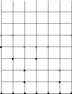
× ×represent a point in the∂S6
• represents a particle inS6
Figure 1: The clusterS6and its boundary.
We consider the L-strip D = [0, L−1]×Z+. We denote the columns by Dl = {l} ×Z+,
l∈ {0, . . . , L−1}. The symbols⊕and⊖stand for addition and subtraction modL. For each pointx= (l, m)∈D we say that (l⊖1, m+ 1),(l, m+ 1) and (l⊕1, m+ 1) are the neighbors of x, and write∂x for this set of neighbors. For a clusterS (namely, a finite subset of D), which intersects all columnsDl,l∈ {0, . . . , L−1}, we define the neighborhood∂S ofS as
∂S={(l, m) :mis the greatest numberm′ for which (l, m′)∈∂x for somex∈S}.
Note that, in each column there is exactly one element of∂S.
We begin with an initial cluster of particles S0 ={0, . . . , L−1} × {0}and for each ndefine
recursivelySn as follows. Let (Ω,F,P) be a probability space on whichLindependent rate 1
Poisson proceses M0, M1, . . . ML−1 are defined. Assume that Ω is given in a canonical form,
i.e ω(t) = (M0(t, ω), M1(t, ω), . . . ML−1(t, ω)). The shift bysoperators{θs, s≥0} act on Ω
in the usual way. Letτn,n= 0,1, . . .be thenth jump time of any of these processes. Namely,
letτ0= 0 and for n≥1 let
τn = inf{t > τn−1:Ml(t)> Ml(τn−1), for somel}.
Let ln be the index of the Poisson process jumping at τn, namely the unique l satisfying
Ml(τn) =Ml(τn−1) + 1. We letyn denote the point where the column Dln intersects ∂Sn−1, and then letSn ={yn} ∪Sn−1. Fort∈[τn, τn+1) we denoteS(t) =Sn. See figure 1.
We say that h is the height of a cluster S at column Dl if h is the greatest number m for
(hl(t), l ∈ {0, . . . , L−1}), t ≥ 0 is a Markov process which can be described as follows. It
changes only at the timesτn and according to
hl(τn) =
1 +hl⊖1(τn−1)∨hl(τn−1)∨hl⊕1(τn−1) l=ln,
hl(τn−1) l6=ln,
(1)
forn= 1,2, . . .. The initial condition is hl(0) = 0,l= 0, . . . , L−1. We also let the maximal
height at timetbe defined as
H(t) = max
0≤l≤L−1hl(t) (2)
Define for 0≤s≤t,H(s, t) =H(t−s)◦θs. In words,H(s, t) is the maximal height at time
t−s, obtained when the model is driven by the processes ˜Mi(t) =Mi(t+s),i= 0, . . . , L−1,
t ≥ 0, rather than the processes Mi(t), i = 0, . . . , L −1, t ≥ 0. It is easy to see that
H(0, s+t)≤H(0, s) +H(s, t) and thatEH(0,1)<∞. By Kingman’s Sub-additive Ergodic Theorem [7] it follows that a.s.,
lim
t→∞t
−1H(t) = lim
t→∞t
−1EH(t) = inf
t>0t
−1EH(t) =:C
L. (3)
One can express the constantCLas a function of the invariant measure of the process{hj⊕1−
hj,0≤j ≤L−1}. However, this measure is not known in an explicit form. We are able to
provide bounds onCL.
Theorem 1.1 For all L≥4,3.21< CL<5.35.
One can dominate the height by that of a model that possesses the same transition law as the above model, except that at each time the maximal height hits a multiple ofL, say kL, the heights at all sitesj= 0, . . . , L−1 are reset tokL. This model gives us the upper bound (in Section 2.1). The lower bound is obtained by analyzing a “slower” model, one for which the growth rate is smaller. The simplest example of a slower model is one in which only events (i.e., particle attachments) that immediately increase the maximal heightH are accepted, and all other events are ignored. This model easily yields a lower bound of 3 onCL. We construct
a slightly more complicated model than the one just described. We discuss it in detail in Section 2.2.
Finally in Section 3, we conclude the paper with remarks detailing interesting connections of this model to some other problems.
2
Proof of Theorem 1.1
2.1
An upper bound
Let m ∈ Z+ be fixed. We define a sequence of stopping times as follows. LetT0 = 0 and forn = 0,1, . . .let Tn+1 = inf{t > Tn : H(Tn, t) = m}. Then T1 is simply the first time the
maximal heightH(·) is equal tom, andTn+1−Tnis the first time the heightH(Tn,·) is equal
to m. By subadditivity we have that H(Tn) ≤ nm. Taking limit on a subsequence in (3)
shows that a.s.,
CL≤ lim n→∞
nm Tn
= m
ET1
where the last equality follows from the facts thatTn+1−Tnare i.i.d.,ET1<∞and the Law
of Large Numbers. We will show that a lower bound onET1 of the order ofmholds.
Fora >0 one has
necessary and sufficient for having H(t)≥n,we have
P(T1< am) = P(
A naive estimate on each term in this sum, not depending on b, is referred to in an aside at the end of this proof. We proceed with a more involved argument. Fix a b ∈ Bm. Let
β =β(b)⊂ {1, . . . , m}be the set ofi for whichbi =bi−1. Similarly letβ+ [resp.,β−] be the
Forbto be a backbone at timeam, it is necessary that the following hold: σm< am; occurrence
of the eventsNk
(where ∆σ is an exp(1) random variable)
= (3 +ν)−|β|(2 +ν)−(m−|β|)eνam. (9)
Next, note that in Bm there are mk
2m−k sequences b with |β(b)| = k. Using the bound
obtained in (9) for eachb∈Bmand from the deduction in (6) we conclude that
Letg(x) =−xlogx−(1−x) log(1−x) forx∈(0,1).Using Sterling’s formula it directly follows that mk
≤cmcexp(mg(k/m)),wherecis a constant independent ofmandk. Therefore (10)
along with this inequality imply that
P(T1< am)≤cmc(m+ 1) exp(mG(ν, a)), (11)
To finish the proof of the upper bound we need the following lemma, proved at the end of this section.
Lemma 2.1 Let a0 be as defined in (14). Then 1/a0<5.35.
Using (11) we can conclude that
lim sup Proof of Lemma 2.1: One finds from (12) that
Aside: One can obtain an upper bound, albeit less sharp, forCL via a simpler but rougher
large deviations estimate. Proceed as indicated in the above proof till (6). Then denote by
Sm, the sum of mi.i.d. standard exponential random variables (si), and forλ >0 arbitrary,
use Chebycheff’s inequality to get
P(T1< am) ≤ L3mP(Sm< am) =L3mP( m
X
1
−si>−am)≤L3meaλm Ee−λs1 m
= L3meaλm
1 1 +λ
m
=Le(aλ−log(1+λ)+log 3)m. (17)
Optimizing over λ gives, at λ = (1−a)/a, the estimate Le(1−a+log 3a)m. Then proceed as
indicated in the proof of Theorem 1.1 after (15) to geta−01<7.1.
2.2
A lower bound
We obtain lower bounds by considering models whose height processes are dominated by that of the model of interest. Recall that the clusters are defined via the recursion
Sn={yn} ∪Sn−1,
whereynis where∂Sn−1intersectsDln. The idea is to modify the recursive definition and let
˜
Sn= [{yn} ∪S˜n−1]∩F(ln, Sn−1), (18)
where F is some function taking values in the set of subsets ofD. Hereyn is where ∂S˜n−1
intersectsDln, and if the intersection is empty, then with an abuse of notation,{yn}is regarded as the empty set.
The caseF ≡Dis equivalent to (1). Suppose we couple our model of interest with the model (18) so that they are defined on the same probability space and so that{τn}and {ln} come
from the same set of Poisson processes. Then by induction, the height in (1) is greater than or equal to the height process associated with (18) for allt≥0 a.s.
The advantage of considering (18) is that one can restrict to a recursion within a set of clusters all of which are vertical shifts of only a finite number of clusters. The simplest example would arise if all clusters are singletons. This corresponds to taking
F(ln,S˜n−1) =
{yn} ∂S˜n−1∩Dln6=∅,
˜
Sn−1 otherwise,
where yn is defined as before. The height in this model grows by 1 each time Dln intersects
∂S˜n−1=∂yn−1. Therefore, the height grows at rate 3, and as a result we get thatCL≥3.
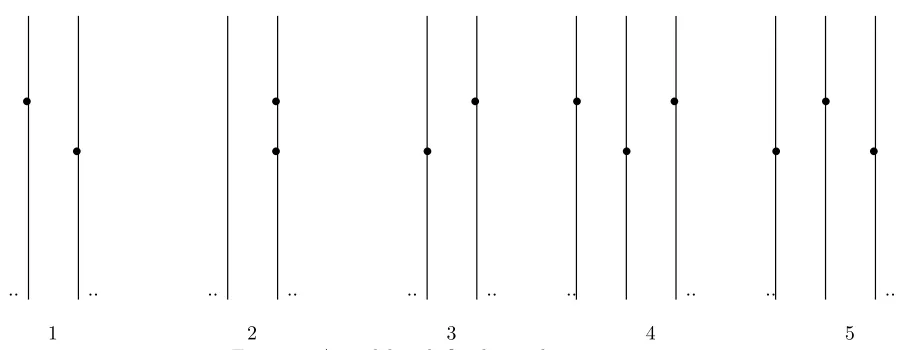
Heuristically, the way in which the above model simplifies (1) is by keeping track of one component and ignoring the events that do not immediately contribute to its growth. In the next model we consider, less such events are ignored. Here ˜Sn takes values in the set of
clusters that are vertical and horizontal shifts of the five ‘basic clusters’ depicted at Figure 2. The precise definition ofF for this model is cumbersome, and is therefore skipped. However, the dynamics of the model should be clear from the following example. Suppose ˜Sn−1 is a
shifted version of cluster 3 (in Figure 2), located at columnsDlandDl+1. Then ifln=l−1,
Similarly, ifln=l, l+ 1, l+ 2, respectively, then Sn will be a shifted version of cluster 1,2,3,
respectively.
One obtains a five state Markov process, which is analyzed as follows. The intensity matrix is
G=
As a result, the growth rate of this model is
3[p(1) +p(2) +p(3) +p(5)] + 5p(4) = 3.21
and we conclude thatCL≥3.21 forL≥4.
A more careful analysis based on a larger number of basic clusters results with a bound of
CL>3.25. Figure 2: A model with five basic clusters
3
Remarks
We remark on some alternative ways to represent the model.
(a)Longest increasing subsequence problem.
The asymptotic of the longest length of an increasing subsequence of a random permutation of
unrelated, we point out that the height in the model discussed here equals the longest length of a subsequence which changes by−1, 0 or 1 of a sequence ofnrandom drawings from{1, . . . , L}.
(b)Products of random matrices.
There is an equivalent formulation of the problem in terms of products of certain random matrices. Forb∈Rconsider theL×LmatricesAl,l= 1, . . . , Lwith
Al(i, j) =
1 i=j6=l,
b i=l, j−l= 0 or ±1 modL,
0 otherwise.
Let Xn be a sequence of i.i.d. random matrices where the law ofX1 is uniform on {Al, l =
1, . . . , L}. ConsiderMn=XnXn−1· · ·X1and letedenote the column vector of lengthLwith
entries 1. Note that theith entryPi(b) of the vectorMneis a polynomial inb. If one considers
a coupling to the model studied in Section 1, in such a way that Xn =Aln for everyn, then one checks that the heighthi(tn) of theith column (wheretn is thenth event) is given by the
degree ofPi. Hence the heightH(tn) is given by the degree of the polynomialP(b) =e′Mne.
Acknowledgments: The work was done when the three of us were visiting the Fields Institute for Research in Mathematical Sciences in Toronto, Canada. We would like to thank the staff for their hospitality, Jeremy Quastel for introducing us to ballistic deposition, Gregory Lawler and Richard Durrett for helpful discussions.
References
[1] M. Barlow, Fractals and diffusion-limited aggregation,Bull. Sc. Math, 117:161-169,1993. [2] M. Barlow, R. Pemantle and E. Perkins, Diffusion-limited aggregation on a tree,
Proba-bility Theory and Related Fields, 107:1-60, 1997.
[3] M. Bramson, D. Griffeath, and G. Lawler. Internal diffusion limited aggregation. The Annals of Probability, 20:2117–2140,1992.
[4] D. Eberz, Ph.D. thesis, University of Washington, 1999.
[5] H. Kesten, How long are the arms in DLA.?,J. Phys. A, 20:L29-L33,1987.
[6] M. Penrose and J. Yukich, Limit theory for random sequential packing and deposition, preprint.