THE SPECTRUM OF THE EDGE CORONA OF TWO GRAPHS∗
YAOPING HOU† AND WAI-CHEE SHIU‡
Abstract. Given two graphsG1, with vertices 1,2, ..., nand edgese1, e2, ..., em, andG2, the
edge coronaG1⋄G2ofG1andG2is defined as the graph obtained by takingmcopies ofG2and for
each edgeek=ijofG, joining edges between the two end-verticesi, j ofekand each vertex of the
k-copy ofG2.In this paper, the adjacency spectrum and Laplacian spectrum ofG1⋄G2 are given
in terms of the spectrum and Laplacian spectrum ofG1 andG2,respectively. As an application of
these results, the number of spanning trees of the edge corona is also considered.
Key words. Spectrum, Adjacency matrix, Laplacian matrix, Corona of graphs.
AMS subject classifications. 05C05, 05C50.
1. Introduction. Throughout this paper, we consider only simple graphs. Let
G= (V, E) be a graph with vertex setV ={1,2, ..., n}. The adjacency matrix ofG
denoted byA(G) is defined asA(G) = (aij),whereaij = 1 ifiandj are adjacent in
G,0 otherwise. The spectrum ofGis defined as
σ(G) = (λ1(G), λ2(G), ..., λn(G)),
where λ1(G) ≤ λ2(G) ≤ ... ≤ λn(G) are the eigenvalues of A(G). The Laplacian
matrix ofG, denoted byL(G) is defined asD(G)−A(G),whereD(G) is the diagonal degree matrix ofG. The Laplacian spectrum ofGis defined as
S(G) = (θ1(G), θ2(G), ..., θn(G)),
where 0 =θ1(G)≤θ2(G)≤... ≤θn(G) are the eigenvalues ofL(G).We call λn(G)
and θn(G) the spectral radius and Laplacian spectral radius, respectively. There is extensive literature available on works related to spectrum and Laplacian spectrum of a graph. See [2, 5, 6] and the references therein to know more.
The corona of two graphs is defined in [4] and there have been some results on the corona of two graphs [3]. The complete information about the spectrum of the corona of two graphsG, H in terms of the spectrum ofG, H are given in [1]. In this
∗Received by the editors September 11, 2009. Accepted for publication August 22, 2010.
Han-dling Editor: Richard A. Brualdi.
†Department of Mathematics, Hunan Normal University, Changsha, Hunan 410081, China
([email protected]). Research supported by NSFC(10771061).
‡Department of Mathematics, Hong Kong Baptist University, Hong Kong, China.
paper, we consider a variation of the corona of two graphs and discuss its spectrum and the number of spanning trees.
Definition 1.1. Let G1 and G2 be two graphs on disjoint sets of n1 and n2
vertices, m1 and m2 edges, respectively. The edge coronaG1⋄G2 ofG1 andG2 is
defined as the graph obtained by taking one copy of G1 and m1 copies of G2, and
then joining two end-vertices of thei-th edge of G1 to every vertex in thei-th copy
ofG2.
Note that the edge corona G1⋄G2 of G1 and G2 has n1+m1n2 vertices and
m1+ 2m1n2+m1m2 edges.
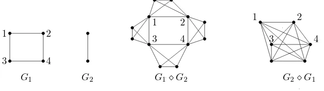
Example 1.2. Let G1 be the cycle of order 4 and G2 be the complete graph
K2 of order 2. The two edge coronasG1⋄G2 andG2⋄G1 are depicted in Figure 1.
G1 G2 G1⋄G2 G2⋄G1
1 2
3 4
1 2
3 4
1 2
[image:2.612.79.409.336.429.2]3 4
Figure 1: An example of edge corona graphs
Throughout this paper, G1 is assumed to be a connected graph with at least
one edge. In this paper, we give a complete description of the eigenvalues and the corresponding eigenvectors of the adjacency matrix of G1⋄ G2 when G1 and G2
are both regular graphs and give a complete description of the eigenvalues and the corresponding eigenvectors of the Laplacian matrix of G1⋄G2 for a regular graph
G1 and arbitrary graph G2. As an application of these results, we also consider the
number of spanning trees of the edge corona.
2. The spectrum of the graph G1⋄G2. Let the vertex set and edge set of a
graph Gbe V ={1,2, ..., n} and E ={e1, e2, ..., em}, respectively. The vertex-edge incidence matrixR(G) = (rij) is an n×mmatrix with entryrij = 1 if the vertex i is incident the edgeej and 0 otherwise.
Lemma 2.1. [2, P. 114] LetGbe a connected graph with nvertices andR be the
vertex-edge incident matrix. Thenrank(R) =n−1ifGis bipartite andnotherwise.
connected bipartite graph with vertex partition V = V1∪V2 and X = (X1, X2)T
is an eigenvector corresponding eigenvalue λ of A(G) then X = (X1,−X2)T is an
eigenvector corresponding eigenvalue−λofA(G).
LetA= (aij), Bbe matrices. Then the Kronecker product ofAandB is defined the partition matrix (aijB) and is denoted byA⊗B. The row vector of sizen with all entries equal to one is denoted byjn and the identity matrix of ordernis denoted byIn.
LetG1andG2be graphs withn1, n2vertices andm1, m2edges,respectively. Then
the adjacency matrix ofG=G1⋄G2 can be written as
A(G) =
A(G1) R(G1)⊗jn2
(R(G1)⊗jn2)
T I
m1⊗A(G2)
,
whereA(G1) andA(G2) are the adjacency matrices of the graphsG1andG2,
respec-tively, andR(G1) is the vertex-edge incidence matrix of G1. A complete
characteri-zation of the eigenvalues and eigenvectors ofG1⋄G2 will be given when bothG1 and
G2are regular.
LetG1be anr1-regular graph andG2be anr2-regular graph and
(2.1) σ(G1) = (µ1, µ2, ..., µn1), σ(G2) = (η1, η2, ..., ηn2)
be their adjacency spectrum, respectively. If G1 is 1-regular then G1=K2 as G1 is
connected. In this case,G1⋄G2is the complete product ofK2andG2.By Theorem 2.8
of [2], or by some direct computations, we can obtain the spectrum ofG=G1⋄G2as
(η1, ..., ηn2−1, µ1=
r2+µ1−
√
(r2−µ1)2+4(r1+µ1)n2
2 ,
r2+µ2±
√
(r2−µ2)2+4(r1+µ2)n2
2 ), where
µ1=−1, µ2= 1 are the spectrum ofK2.
Theorem 2.3. Let G1 be an r1-regular (r1 ≥2) graph andG2 be an r2-regular
graph and their spectra are as in (2.1). Then the spectrumσ(G)of Gis
Ã
η1 η2 · · · ηn2=r2
r2+µ1±
√
(r2−µ1)2+4(r1+µ1)n2
2 · · ·
m1 m1 · · · m1−n1 1 · · ·
r2+µn1±√(r2−µn1)2+4(r1+µn1)n2
2
1
!
G2 G2 G2 G2 G2 G1 0 0 ei Zj 0 Xi s t
Xi(u)+Xi(v) λi−r2 j
u v G1 s t u v
Yuvj G1
G2
G2 0
Figure 2: Description of adjacency eigenvectors
Proof. LetZ1, Z2, ..., Zn2 be the orthogonal eigenvectors ofA(G2) corresponding
to the eigenvalue η1, η2, ..., ηn2 = r2, respectively. Note that G2 is r2-regular and
Zj⊥j for j = 1,2, ..., n2−1. Then for i = 1,2, ..., m1 and for j = 1,2, ..., n2−1,
we have (see Figure 2, picture on the left) that (n1 +m1n2)-dimension vectors
(0,0, ...,0, Zj,0, ...,0)T,where (i+1)-th block isZjare eigenvectors ofGcorresponding to eigenvalueηj.Thus we obtainm1(n2−1) eigenvalues and corresponding
eigenvec-tors ofG.
LetX1, X2, ..., Xn1 be the orthogonal eigenvectors ofA(G1) corresponding to the
eigenvaluesµ1, µ2, ...µn1, respectively. Fori= 1,2, ..., n1, let
λi=
r2+µni+
p
(r2−µni)
2+ 4(r
1+µni)n2
2 and
λi=
r2+µni−
p
(r2−µni)
2+ 4(r
1+µn−)n2
2 .
Note that r2+µni±√(r2−µni)2+4(r1+µni)n2
2 =r2if and only ifµi =−r1.Soλiorλiisr2
if and only ifG1is bipartite (note that at most one ofλiisr2). IfG1is bipartite and
the bipartition of its vertex set isV1∪V2,then by Lemma 2.2 and some computations,
we obtain that (j,−j,0, ...,0)T (1 onV
1,−1 onV2, and 0 on all copies of G2 ) is an
eigenvector ofGcorresponding the eigenvalue −r1.
Observe that if λi and λi are not equal to r2 then λi and ¯λi are eigenval-ues of G corresponding to the eigenvectors Fi = (Xi, ...,X
i(s)+Xi(t)
λi−r2 , ...)
T and F
i =
(Xi, ...,X
i(s)+Xi(t)
λi−r2 , ...)
T,respectively (see Figure 2, picture in the middle). In fact, it
needs only to be checked that characteristic equations P
v∼uFi(v) =λiFi(u) (resp. P
v∼uF¯i(v) =λiF¯i(u)) hold for every vertexuin G.
For any vertex u in k-copy of G2, let edge ek = st, then Fi(u) = X
i(s)+Xi(t)
λi−r2 .
Furthermore,
X
v∼u
For any vertexuinG1,
X
v∼u
Fi(v) = X v∼u,v∈V(G1)
Fi(v) + X v∼u,v6∈V(G1)
Fi(v)
=µiXi(u) +
r1n2Xi(u)
λi−r2
+ n2
λi−r2
X
v∼u,v∈V(G1)
Fi(v)
=λiXi(u) =λiFi(u).
Therefore we obtain 2n1 eigenvalues and corresponding eigenvectors of G ifG1
is not bipartite and 2n1−1 eigenvalues and corresponding eigenvectors of GifG1 is
bipartite.
LetY1, Y2, ..., Ybbe a maximal set of independent solution vectors of linear system
R(G1)Y = 0. Thenb =m1−n1 ifG1 is not bipartite andb=m1−n1+ 1 ifG1 is
bipartite. Fori= 1,2, ..., b,letHi= (0, Yi(e1)j, ..., Yi(em)j)T (see Figure 2, picture on
the right). We can obtain thatHi is an eigenvector ofGcorresponding to eigenvalues
r2=ηn2.Thus theseY
′
isprovideb eigenvalues and corresponding eigenvectors ofG.
Therefore we obtainn1+m1n2 eigenvalues and corresponding eigenvectors ofG
and it is easy to see that these eigenvectors ofGare linearly independent. Hence the proof is completed.
Next we consider the Laplacian spectrum ofG1⋄G2.
Let L(G1) and L(G2) be the Laplacian matrices of the graphs G1 and G2,
re-spectively, andR(G1) be the vertex-edge incidence matrix ofG1.Then the Laplacian
matrix ofG=G1⋄G2is
L(G) =
L(G1) +r1n2In1 −R(G1)⊗jn2
−(R(G1)⊗jn2)
T I
m1⊗(2In2+L(G2))
.
In the following, we give a complete characterization of the Laplacian eigenvalues and eigenvectors ofG1⋄G2.
LetG1be anr1-regular graph andG2be any graph and
(2.2) S(G1) = (θ1, θ2, ..., θn1), S(G2) = (τ1, τ2, ..., τn2)
be their Laplacian spectra, respectively. If G1 is 1-regular then G1 =K2 as G1 is
connected. In this case,G1⋄G2is the complete product ofK2andG2 (by [5]), or by
is
S(G) = (0, τ2+ 2, ..., τn2+ 2, n2+ 2, n2+ 2 ).
Theorem 2.4. Let G1 be anr1-regular (r1≥2) graph andG2 be any graph and
their Laplacian spectra are written as in (2.2). Let
βi,β¯i=
r1n2+θi+ 2± p
(r1n2+θi+ 2)2−4(n2+ 2)θi 2
for everyθi. Then the Laplacian spectrum S(G)of Gis
µ
τ1+ 2, τ2+ 2, · · · , τn2+ 2, β1, β¯1, · · ·, βn1, β¯n1
m1−n1 m1 · · · m1 1 1 · · · 1 1 ¶
where entries in the first row are the eigenvalues with the number of repetitions written below, respectively.
G2
G2
G2
G2
G2
G1
0
0
ei
Zj
0
Xi s t
Xi(s)+Xi(t) 2−βi j
Xi(u)+Xi(v) 2−βi j
u v
G1
s t
u v
Ystj
Yuvj
G1
G2
G2 0
Figure 3: Description of Laplacian eigenvectors
Proof. LetZ1, Z2, ..., Zn2be the eigenvectors ofL(G2) corresponding to the
eigen-values 0 =τ1, τ2, ..., τn2.Note thatZj⊥jforj= 2, ..., n2.Then fori= 1,2, ..., m1 and
forj = 2,3, ..., n2, we have that (n1+m1n2)-dimension vectors (0,0, ...,0, Zj,0, ...,0)T, where (i+1)-th block isZjare eigenvectors ofL(G) corresponding to eigenvalueτj+2 (see Figure 3, picture on the left). Thus we obtainm1(n2−1) eigenvalues and
corre-sponding eigenvectors ofL(G).
LetX1, X2, ..., Xn1 be the orthogonal eigenvectors ofL(G1) corresponding to the
eigenvaluesθ1, θ2, ..., θn1,respectively. Fori= 1,2, ..., n1,note that:
βi,β¯i=
r1n2+θi+2±√(r1n2+θi+2)2−4(n2+2)θi
2 =
r1n2+θi+2±√(r1n2+θi−2)2+4n2(2r1−θi)
2
sincer1 ≥2, n2 ≥1, βi 6= 2. Note that θi ≤2r1 and the equality holds if and only
if G1 is bipartite. Note that ¯βi = 2 implies that θi = 2r1. That is, ¯βi = 2 appears only if G1 is bipartite and i = n1. Moreover, if G1 is bipartite and the bipartition
−1 onV2, and 0 on all copies of G2) is an eigenvector corresponding the eigenvalue
(n1+ 2)r1=βn1 ofL(G).
Observe that ifβiand ¯βiare not equal to 2, thenβiand ¯βiare eigenvalues ofL(G) andFi = (Xi, ...,X
i(s)+Xi(t)
2−βi , ...)
T and ¯F
i = (Xi, ...,X
i(s)+Xi(t)
2−βi
, ...)T are eigenvectors ofβi and ¯βi respectively (see Figure 3, picture in the middle). In fact, it needs only to be checked that characteristic equationsdG(u)Fi(u)−P
v∼uFi(v) =βiFi(u) (resp.
dG(u) ¯Fi(u)−P
v∼uF¯i(v) = ¯βiF¯i(u)) hold for every vertexuinG,wheredG(u) is the degree of the vertexuin G.
For every vertexuink-copy ofG2,let the edgeek =st,thendG(u) =dG2(u) + 2
andFi(u) = Xi(s)+Xi(t)
2−βi . Further,
dG(u)Fi(u)−X
v∼u
Fi(v) =dG2(u) + 2)Fi(u)−dG2(u)
Xi(s) +Xi(t)
2−βi −
(Xi(s) +Xi(t))
=βiFi(u).
For every vertexuin G1,note that
r1Xi(u)− X
v∼u v∈V(G1)
Xi(v) =θiXi(u).
We have
dG(u)Fi(u)− X
v∼u
Fi(v) = (r1+r1n2)Fi(u)−
X
v∼u,v∈V(G1)
Fi(v) +
X
v∼u,v6∈V(G1)
Fi(v)
= (r1+r1n2)Xi(u)−
X
v∼u,v∈V(G1)
Xi(v)− X
v∼u,v∈V(G1)
n2
2−βi
(Xi(u) +Xi(v))
= (r1+r1n2)(2−βi)−2n2r1+n2θi 2−βi
Xi(u) + (θi−r1)Xi(u)
=βiXi(u) =βiFi(u).
Therefore we obtain 2n1 eigenvalues and corresponding eigenvectors of L(G) if
G1 is not bipartite, and 2n1−1 eigenvalues and corresponding eigenvectors ofL(G)
ifG1 is bipartite.
Let Y1, Y2, ..., Yb be a maximal set of independent solution vectors of the linear systemR(G1)Y = 0. Thenb=m1−n1 ifG1 is not bipartite, andb=m1−n1+ 1
if G1 is bipartite. For i = 1,2, ..., b, let Hi = (0, Yi(e1)j, ..., Yi(em)j)T (see Figure
Therefore we obtain n1+m1n2 eigenvalues and corresponding eigenvectors of
L(G) and it is easy to see that these eigenvectors ofL(G) are linearly independent. Hence the proof is completed.
As an application of the above results, we give the number of spanning trees of the edge corona of two graphs.
LetGbe a connected graph withnvertices and Laplacian eigenvalues 0 =θ1<
θ2≤ · · · ≤θn.Then the number of spanning trees of Gis
t(G) =θ2θ3· · ·θn
n .
By Theorem 2.4 we have
Proposition 2.5. For a connectedr1-regular graph G1 and arbitrary graphG2,
let the number of spanning trees of G1 be t(G1) and the Laplacian spectra of G2 be
0 =τ1≤τ2≤ · · · ≤τn2.Then the number of spanning trees of G1⋄G2 is
t(G1⋄G2) = 2m1−n1+1(n2+ 2)n1−1t(G1)(τ2+ 2)m1· · ·(τn2+ 2)
m1.
Proof. Following the notions in Theorem 2.4, note that βiβ¯i = (n2+ 2)θi for
i= 1,2, ..., n1 andβ1=r1n2+ 2,β¯1= 0.Thus
t(G1⋄G2) =
2m1−n1(r
1n2+ 2)(n2+ 2)n1−1Qin=22 (τi+ 2)m1Qnj=21 θj
n1+m1n2
= n12
m1−n1(r
1n2+ 2)(n2+ 2)n1−1t(G1)Qni=22 (τi+ 2)m1
n1+m1n2
= 2m1−n1+1(n
2+ 2)n1−1t(G1)(τ2+ 2)m1· · ·(τn2+ 2)
m1.
The last equality follows fromn1+m1n2=n1(2+2r1n2).
By Proposition 2.5, we have t(G⋄K1) = 2m−n+13n−1t(G) for a regular graph
G.In factt(G⋄K1) = 2m−n+13n−1t(G) holds for arbitrary graphGby the following
proposition.
Proposition 2.6. LetGbe a connected graph withnvertices andmedges. Then the number of spanning trees ofG⋄K1is2m−n+13n−1t(G),wheret(G)is the number
of spanning trees of G.
Proof. Note that the Laplacian matrix ofG⋄K1is
L(G⋄K1) = µ
L(G) +D(G) −R
−RT 2I m
¶
Let (L(G))11 be the reduced Laplacian matrix of G obtained by removing the
first row and first column of L(G) andR1 be the matrix obtained by removing the
first row of the vertex-edge incidence matrixR.By the Matrix-Tree theorem [2], we have
t(G⋄K1) = det(L(G⋄K1))11= det µ
(L(G) +D(G))11 −R1 −RT
1 2Im
¶
= 2mdet[(L(G) +D(G))
11−
1 2R1R
T
1],
sinceRRT =D(G) +A(G), R
1R1T = (D(G) +A(G))11.Thus
t(G⋄K1) = 2mdet(
3
2(D(G)−A(G))11= 2
m−n+13n−1
t(G).
Acknowledgments. The authors would like to express their sincere gratitude to the referee for a very careful reading of the paper and for all his or her insightful comments and valuable suggestions, which made a number of improvements on this paper
REFERENCES
[1] S. Barik, S. Pati, and B. K. Sarma. The spectrum of the corona of two graphs. SIAM. J. Discrete Math.,24:47–56, 2007.
[2] D. Cvetkovi´c, M. Doob, and H. Sachs. Spectra of Graphs: Theory and Application,Johann Ambrosius Barth Verlag, Heidelberg-Leipzig, 1995.
[3] R. Frucht and F. Harary. On the corona two graphs.Aequationes Math.,4:322–325, 1970.
[4] F. Harary. Graph Theory. Addition-Wesley Publishing Co., Reading, MA/Menlo Park,
CA/London, 1969.
[5] R. Merris. Laplacian matrices of graphs: a survey. Linear Algebra Appl., 197/198:143–176, 1994.