Gregory T. Niemesh is an assistant professor of economics at Miami University. Research on this project was generously supported by the John E. Rovensky Fellowship, the Vanderbilt University Summer Research Awards Program in Arts and Science, Graduate School Dissertation Enhancement Program, Noel Disserta-tion Fellowship, and Kirk Dornbush Summer Research Grant. He is grateful to William J. Collins, Jeremy Atack, Kathryn Anderson, Douglas C. Heimburger, Hoyt Bleakley, Martha Bailey, Alan Barreca, and to discussants and seminar participants at UC- Davis, University of Michigan, Colgate University, Miami University, the 2011 Cliometrics Conference, Population Association of America Meetings, the NBER Summer Institute, and the Economic History Association Annual Meetings. The data used in this article can be obtained beginning March 2016 through April 2019 from Gregory Niemesh, 800 E. High Street, Oxford Ohio, niemesgt@miamioh.edu.
[Submitted July 2013; accepted July 2014]
ISSN 0022- 166X E- ISSN 1548- 8004 © 2015 by the Board of Regents of the University of Wisconsin System
T H E J O U R N A L O F H U M A N R E S O U R C E S • 50 • 4
Ironing Out De
fi
ciencies
Evidence from the United States on the
Economic Effects of Iron De
fi
ciency
Gregory T. Niemesh
NiemeshABSTRACT
Iron defi ciency reduces productive capacity in adults and impairs cognitive development in children. In 1943, the United States government required the fortifi cation of bread with iron to reduce iron defi ciency in the working- age population during World War II. This nationwide fortifi cation of grain products increased per capita consumption of iron by 16 percent. I fi nd that areas with lower levels of iron consumption prior to the mandate experienced greater increases in income and school enrollment in the 1940s. A long- term followup suggests that adults in 1970 with more exposure to fortifi cation during childhood earned higher wages.
I. Introduction
impact of health interventions on productivity and quality of life.1 For instance, the Copenhagen Consensus of 2008 recommends iron and iodine fortifi cation as a highly cost- effective development intervention (Lomborg 2009). Although fortifi cation pro-grams diffused rapidly after the fi rst implementation in the early 1940s, signifi cant potential remains for further gains. As of 2009, 63 countries had implemented fl our fortifi cation programs, but 72 percent of world refi ned fl our production remained un-fortifi ed (Horton, Mannar, and Wesley 2008).
Surprisingly few studies directly evaluate the effects of national- level fortifi cation programs. Of those that do, data limitations and experimental design issues limit their usefulness for policy. Layrisse et al. (1996) fi nd reductions in anemia and defi ciency rates from a 1993 Venezuelan program but no control group was used as a comparison and no economic outcomes were included in the analysis. Imhoff- Kunsch et al. (2007) use expenditure data to measure the potential for improvements in health based on reported consumption of fortifi ed foods but do not directly evaluate health or eco-nomic outcomes in response to the intervention. In practice, estimates of benefi t- cost ratios for iron fortifi cation typically proceeded by applying productivity estimates from supplementation fi eld trials to prevalence measures from health surveys (Horton and Ross 2003).
This paper uses a sweeping change in federal policy in the United States in the 1940s to estimate both the short- term and long- term effects of fortifi cation on labor market outcomes and human capital development. The discovery of vitamins and min-erals during the early 20th century intensifi ed the public health profession’s interest in the nutritional status of Americans. A number of diet surveys and blood serum case studies during the 1930s showed a widespread prevalence of defi ciencies in iron.2 Low iron consumption was found in all socioeconomic classes but the prevalence varied across geographic areas. For example, one study found that the proportion of the population considered iron defi cient ranged from 47 and 74 percent of white and African- American children in a rural Tennessee county to less than 5 percent of adult male aircraft manufacturing workers in southern California (Kruse et al. 1943; Bor-sook, Alpert, and Keighley 1943). Taking the case studies as a whole, the United States in the 1930s had rates of iron defi ciency similar to those currently found in Turkey or Brazil (de Benoist et al. 2008). Concerns with worker health and production during World War II fi nally led to a national fortifi cation program in 1943, but to my knowl-edge no formal evaluation has tested whether the program led to productivity gains.
In addition to the literature on health and micronutrient fortifi cation in develop-ing countries, this investigation ties to two other branches of research in economics. First, economic historians have linked improvements in nutrition to gains in income
The Journal of Human Resources 912
and health over the last three centuries (Fogel 1994, Floud et al. 2001, Steckel 1995). This literature has mainly focused on calorie and protein malnutrition to the exclusion of the hidden hunger of micronutrient defi ciencies. Unfortunately, the evolving and complex interaction of dietary trends, mortality, and income tends to obscure clear causal interpretations of the cotrending relationships in this literature. Second, applied microeconomists have linked health and productivity outcomes in individual- level data sets. A key theme of this literature is that isolating the causal impact of health is diffi cult but essential (Strauss and Thomas 1998, Almond and Currie 2011). In this paper, I follow a strand of this literature that uses targeted public health interventions to estimate the impact of health on economic outcomes (Bleakley 2007; Feyrer, Politi, and Weil 2013; Cutler et al. 2010; Field, Robles, and Torero 2009).
The paper’s central empirical questions are whether places with relatively low iron consumption levels before the program’s implementation experienced relatively large gains in labor market and schooling outcomes after the program’s implementation, and, if so, whether this pattern can be given a causal interpretation. The identifi ca-tion strategy relies on three main elements. First, as shown in diet surveys from the 1930s, there were signifi cant preexisting differences in iron consumption levels and the prevalence of defi ciency across localities. These differences are only weakly cor-related with preintervention income. Second, the timing of the federal mandate was determined by wartime concerns and technological constraints in the production of micronutrients. In this sense, the timing was exogenous. Finally, iron consumption has a nonlinear effect on health. Therefore, a program that increases iron consumption across the entire population is likely to have disproportionate effects on the health of those who were previously iron defi cient (Hass and Brownlee 2001).
Evaluating this particular program entails a number of data challenges. The ideal data set would observe pre and postfortifi cation nutrition, health outcomes, and eco-nomic outcomes in longitudinal microlevel data. But this ideal data set does not exist. My approach combines the necessary pieces from a number of different sources. The “Study of Consumer Purchases in the United States, 1935–1936” provides detailed diet records and location information for households (ICPSR, USDOL 2009). I then use the U.S. Department of Agriculture National Nutrient Database (USDA 2009) to convert the diets into the associated nutritional intakes. Labor market and school-ing outcomes come from the 1910–50 decennial census microdata (IPUMS, Ruggles et al. 2010). The data sets can be linked at the level of “state economic area” (SEA), essentially a small group of contiguous counties with similar economic and social characteristics circa midcentury.3
I fi nd that after the iron fortifi cation mandate in 1943, wages and school enrollment in areas with low iron intake did increase relative to other areas between 1940 and 1950. The regression results are generally robust to the inclusion of area fi xed effects, regional trends, demographic characteristics, World War II military spending, and Depression- era unemployment. One standard deviation less iron consumption before the program is associated with a 1.9 percent relative increase in male wages from
1940 to 1950, and a one to 1.5 percentage point relative increase in school enroll-ment. These estimates are economically signifi cant, accounting for 3.9 percent and 25 percent of the gains in real income and school enrollment over the decade in areas that started below the median level of iron consumption. I estimate a benefi t- cost ratio of at least 14:1, which is within the range for those estimated in developing countries (Horton and Ross 2003).
I use the 1970 census microdata to undertake a separate analysis that suggests that iron defi ciency had a lasting long- term impact on human capital formation and wages. The cohort analysis measures differences in childhood exposure to fortifi cation by combining differences in years of potential exposure (based on year of birth) with geographic differences in preexisting rates of iron defi ciency (based on place of birth). Cohorts with more exposure to fortifi cation had higher earnings and were less likely to be considered living in poverty by the census. Moving from no exposure to a full 19 years of exposure implies a 2.9 percent increase in earnings as an adult. Increased quantity of schooling does not drive the increase in adult incomes.4
II. Iron De
fi
ciency and the Forti
fi
cation
of Flour and Bread
A. Health Effects of Iron Defi ciency
Iron defi ciency is the most common nutritional defi ciency worldwide and is caused by low dietary intake, blood loss, growth, pregnancy, and impaired absorption. Iron has two main functions in the body: to transport oxygen throughout the body in the blood-stream and to process oxygen in the cells of muscles and tissue.5 A lack of iron causes reduced work capacity through a diminished ability to move oxygen throughout the body and a reduction in the tissue cell’s ability to process oxygen. The reduction in oxygen manifests as reduced aerobic capacity, endurance, energetic effi ciency, vol-untary activity and work productivity (Hass and Brownlee 2001).6 A lack of iron also affects productivity by reducing cognitive ability and skill acquisition.
Iron defi ciency in infants and children causes developmental delays and behav-ioral disturbances, including decreased motor activity, social interaction, and attention (Beard and Connor 2003). Studies that follow the same children over time have found that iron defi ciency can have long- lasting effects on neural and behavioral develop-ment of children even if the defi ciency is reversed during infancy (Lozoff et al. 2006).
4. Assessing the impact with randomized trials would prove diffi cult. The cost of tracking infants into adult-hood and the ethical concerns about withholding treatment over an extended period of time would both prove prohibitive. An historical accident provides the necessary variation in exposure during childhood for the current analysis.
5. Daily iron requirements vary signifi cantly by age and sex. The recommended daily allowance (RDA) for adult men is 8 mg per day whereas the RDA for nonpregnant women of childbearing age is 18 mg per day. No differences in requirements exist between the genders during childhood, but requirements increase during periods of growth. The RDA from childhood to puberty ranges from seven to 11 mg per day (Institute of Medicine 2001).
The Journal of Human Resources 914
Between the ages of 12 and 18, adolescents are at higher risk because of increased iron requirements. The risk subsides by the end of puberty for males but menstruation keeps the risk high for women throughout the childbearing years. In treatment- control studies on subjects with iron defi ciency or anemia, cognitive ability and work capac-ity in adolescents treated with iron therapy improved relative to the placebo group (Groner et al. 1986; Sheshadri and Gopaldas 1989; Seomantri, Politt, and Kim 1985). Poor health during childhood can lead to a reduction in educational investment. Bo-bonis, Miguel, and Puri- Sharma (2006) fi nd an economically large impact of iron supplementation on preschool participation in a developing country context with a 69 percent baseline rate of iron defi ciency.
B. The Fortifi cation Movement and Federal Mandate
Before the intervention in the early 1940s, iron in the U.S. food supply was gradu-ally declining as consumers reduced grain consumption and increased sugar and fat consumption (Gerrior, Bente, and Hiza 2004). While acknowledging that the diets of many Americans were defi cient in micronutrients in the early 20th century, the medi-cal profession and regulatory authorities were initially steadfast in their opposition to the addition of any foreign substances to food products (Wilder and Williams 1944). The Food and Drug Administration (FDA) and the American Medical Association (AMA) reversed views in the 1930s during the debates over whether to allow Vitamin D- fortifi ed milk as a tool to prevent rickets. In an important step for proponents of iron fortifi cation, the AMA backed proposals to enrich bread and fl our with iron and thiamin in 1939 (Bing 1939).
In May 1941, the FDA enacted regulations specifying the labeling of “enriched” wheat fl our. No standard for bread was promulgated at the time. This did not require manufacturers to fortify their products, only that to use the label “enriched fl our” the product must contain between 6 and 24 milligrams of iron and niacin and 1.66 to 2.5 milligrams of thiamin in each pound of fl our (FDA Federal Register 1941). These levels represent a doubling to tripling of the micronutrient content of unenriched prod-ucts. Two years later, the FDA increased the minimums and maximums for enriched fl our (FD Federal Register 1943). During this period, the National Research Council (NRC) promoted enrichment on a voluntary basis for bakers and millers. Anecdotal evidence from the NRC archives suggests that 75 to 80 percent of fl our and bread was voluntarily enriched by 1942 (Wilder and Williams 1944). Most parts of the United States had very high participation rates but the South lagged behind, enriching only 20 percent of the fl our consumed.
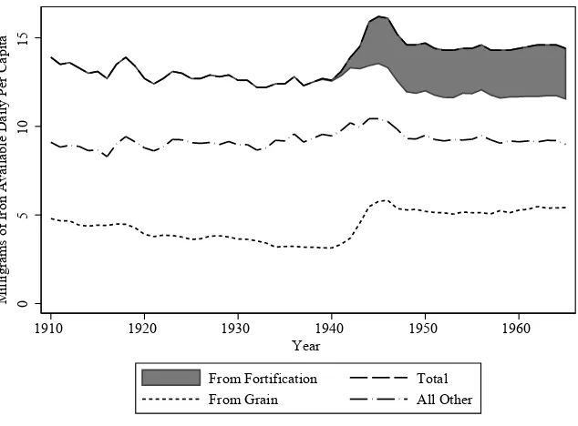
The fi rst federal requirement to fortify bread came in War Food Order Number 1 in 1943, which mandated fortifi cation at the “enriched” levels.7 The mandate had a large, abrupt, and long- lasting impact on iron consumption in the United States. Figure 1 shows a 16 percent increase in the iron content of the U.S. food supply in the early 1940s, which is directly linked to the fortifi cation of fl our and bread.8 By 1950, fortifi -cation provided 22 percent of all iron in the food supply, adding 2.7 milligrams daily.
7. Flour fortifi cation continued on a voluntary basis.
This increase by itself is 34 percent of the recommended daily allowance for men and 15 percent for women. The long secular decline in average iron consumption would have continued unabated into the 1950s in the absence of the intervention.9
III. Identifying the Economic Impact of Iron De
fi
ciency
At the heart of this paper is health’s role as an input into productivity and human capital accumulation. As such, health enters the production function for academic skill, wage equations, or labor supply choice as an input.10 Experiments in the lab often estimate a parameter that approaches the marginal effect of health in the production function for productivity by directly measuring physical work capacity (Rowland et al. 1988, Zhu and Hass 1998, Perkkio et al. 1985). More commonly, a fi eld study provides supplementation for a short period of time and then observes pro-ductivity in jobs where output can be directly measured (Edgerton et al. 1979, Ohira et al. 1979, Gardner et al. 1975).9. Britain also experienced a decline in the iron availability of the food supply during the late- 19th and early- 20th centuries (Barker, Oddy, and Yudkin 1970).
10. See Glewwe and Miguel (2008) and Strauss and Thomas (1998) for a detailed description of the com-monly used model.
0
5
10
15
Milligrams of Iron Available Daily Per Capita
1910 1920 1930 1940 1950 1960
Year
From Fortification Total
From Grain All Other
Figure 1
Historical Iron Levels in the United States Food Supply, 1910–65
The Journal of Human Resources 916
When these estimates are then used to measure cost effectiveness of a policy, po-tential behavioral responses are not taken into account, but they should be.11 People have the choice to adjust inputs along all margins in response to treatment while fac-ing countervailfac-ing income and substitution effects. Behavioral responses can either attenuate or strengthen the effect beyond that of the direct structural effect of the production function relationship. In any case, policymakers usually are not ultimately interested in the structural effect per se; rather, the impact of a health intervention on economic outcomes after taking into account all behavioral adjustments is most useful for informing policy. The estimated effect of iron fortifi cation on school enrollment and income should be interpreted while keeping in mind that adjustments may be made along other margins.
The implementation of the U.S. food fortifi cation program may provide plausibly exogenous variation in health improvements during the 1940s. The empirical strategy relies on three key elements: preexisting differences in iron consumption and preva-lence of defi ciency, exogenous timing of the federal mandate, and the nonlinear effect of iron consumption on health. Assigning a causal interpretation to the partial correla-tions between preprogram iron consumption and subsequent outcomes requires the absence of unobserved shocks and trends to outcomes that are correlated with prepro-gram iron consumption. Such shocks and trends are impossible to rule out completely, but further investigation suggests that the identifying assumption is tenable and that the regression estimates are likely to refl ect a causal relationship.
First, diet surveys and blood sample case studies demonstrated the widespread but uneven prevalence of iron defi ciency across the country in the 1930s. There was considerable variation across places, even within regions. A key concern is whether preprogram iron consumption is highly correlated with income, which could indicate a severe endogeneity problem. Figure 2 demonstrates that a strong relationship does not exist between iron consumption and income during the preprogram period at the SEA level.12 A regression that controls for differences in black proportion of the popula-tion, home ownership, farm status, and the local Gini coeffi cient also shows a weak relationship between income and iron consumption.13 In sum, current local economic characteristics are not strong predictors of preprogram iron consumption, and in any case, regressions below will include controls for income in 1936, local fi xed effects, regional trends, and more.
A signifi cant portion of geographic variation in iron consumption remains unex-plained given that income and demographic characteristics are not good predictors. Contemporaneous price variation explains half the variation. A full explanation of the variation in iron consumption can be thought of as an answer to “Why do people eat what they eat?”—a question outside the scope of this paper. However, the inability of contemporaneous economic variables, especially income, to explain variation in diets
11. Thomas et al. (2006) account for a number of behavioral adjustments in response to an iron supplementa-tion randomized control trial in Indonesia.
is not a novel fi nding (Behrman and Deolalikar 1987, Logan and Rhode 2010). Rela-tive prices from the past predict food consumption 40 years after the fact due to the process of taste formation (Logan and Rhode 2010). Research on the psychology of food and tastes provides further evidence for the importance of learning and the persis-tence of diets (Capaldi 1996). In sum, a number of hypotheses exist in economics and psychology that explain dietary choices based on factors other than current income.
The second piece of the identifi cation strategy comes from the timing of the federal mandate. Its passage was external to what was going on in the low- iron- consumption areas. Fortifi cation was mandated at the federal level in response to wartime concerns, reducing the scope for states, counties, and individual consumers to select into or out of treatment. Moreover, technological constraints made earlier implementation infeasible. The mandate clearly, quickly, and signifi cantly increased per capita iron consumption by 16 percent (Gerrior, Bente, and Hiza 2004).
Finally, iron consumption has a nonlinear effect on health. Above a certain thresh-old, additional iron consumption provides no health improvement—the excess simply gets fi ltered out of the body. Furthermore, severity of defi ciency matters. Gains in health per unit of additional iron are proportional to the extent of the defi ciency (Hass and Brownlee 2001). A nonlinear effect implies that those with low preprogram iron
6
8
10
12
14
16
Average SEA Daily Iron Consumptin in mg
0 1000 2000 3000
Average SEA Income in 1936
Figure 2
Income Only Weakly Predicts Iron Consumption for State Economic Areas
The Journal of Human Resources 918
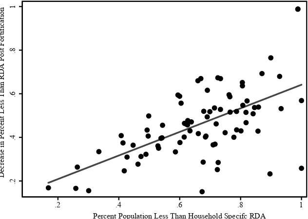
consumption likely experienced larger improvements in health from fortifi cation, even if fortifi cation raised everyone’s intake of iron. This nonlinearity at the individual level translates into differential changes in defi ciency rates at the level of geographic areas. Figure 3 shows that state economic areas with relatively high levels of iron defi ciency before the intervention experienced relatively large declines in defi ciency after the intervention.
Thus, the federal mandate provides a quasi- experiment in which the “treatment effect” varies across areas based on preintervention iron consumption. With census microdata, I estimate equations at the individual level of the following general form, (1) Yits =⋅(IRONs×POSTt)+␦t+␦s+(␦r×t)+Xit1+ Xst2+its
where Y signifi es a labor market or schooling outcome, and δt and δs signify a set of year dummies and state economic area (SEA) indicators. Some specifi cations include a geographic- area- specifi c linear time trend (␦r×t) at the level r, where r denotes
census divisions or SEAs depending on the span of time observed.14 All regressions include a vector of individual- level controls denoted by Xit, with some specifi cations also including a vector of area- specifi c controls denoted by Xst.
The coeffi cient of interest is β. The variable IRONs denotes the preintervention average iron consumption in area s. Each individual is assigned the average prepro-gram iron consumption level for the SEA of residence. The variable POSTt denotes an indicator equal to one if year t is after the intervention date of 1943. Interacting the two gives the variable of interest.15 The hypothesis is that areas with low iron consumption before the intervention experienced larger health benefi ts from fortifi cation and there-fore larger gains in labor market and schooling outcomes. If the hypothesis is correct, then estimates of β should be negative.
Potential threats to a causal interpretation of estimates of β include a trend in or unobserved shock to the outcome that is correlated with preprogram iron consump-tion and is not absorbed by the control variables (Xit and Xst) or place- specifi c trends. I explore potential confounding factors further in the respective estimation section for each outcome.
IV. Diet Data and Preexisting Differences in
Micronutrient Consumption
A. Preintervention Iron Intake and the Study of Consumer Purchases
I use the wealth of household diet information contained in the “Study of Consumer Purchases in the United States, 1935–1936” to calculate household iron consumption and defi ciency as well as average iron consumption for states and state economic areas. The Data Appendix 4 provides an in- depth discussion of the process used to
14. When income is the outcome of interest, the place- specifi c trends cannot be specifi ed at the SEA level because the census started inquiring about income in 1940. This restricts analysis to a two- period comparison (1940 and 1950). However, β can still be identifi ed in regressions that include census- division trends (there are nine census divisions). The census has collected information on school attendance over a longer time span, which allows separate identifi cation of SEA- specifi c trends and β.
construct the iron consumption measure.16 The food schedule portion of the survey provides a detailed account of the types, quantities, and cost of all foods consumed over seven days for a sample of 3,545 households from across the United States.17 The survey contains a surprising amount of detail on the food purchase and consumption patterns of the respondents: Over 681 individual food items are recorded as well as the number of meals provided for each member of the household. The survey included families in 51 cities (population of 8,000 and up), 140 villages (population of 500 to 3,200), and 66 farm counties across 31 states.
Each household diet is converted to iron intake by employing the USDA National Nutrition Database (USDA 2009). I calculate the average daily per person iron
con-16. Work relief, direct relief, or an income below $500 for the largest cities and $250 for other cities caused a household to be ineligible for the expenditure schedule. I assess the size of potential bias from an unrep-resentative sample of diets in the Appendix. The evidence suggests that the fi ndings in the main text are not sensitive to the nonclassical measurement error of dietary iron intake.
17. Total iron intake is equivalent to dietary intake for the vast majority of individuals during this period. Iron supplements as an “insurance policy” were fi rst introduced by the One- A- Day brand in 1965. An iron supple-ment, in conjunction with Vitamins A and D, was marketed at cosmetic counters to middle- class women in the late 1930s as a beauty product. At $33, a year supply was expensive for the average household in my sample with an income of $904 (Apple 1996).
.2
.4
.6
.8
1
Decrease in Percent Less Than RDA Post Fortification
.2 .4 .6 .8 1
Percent Population Less Than Household Specifc RDA
Figure 3
State Economic Areas with Higher Rates of Inadequate Diets in 1936 Experienced Larger Reductions in Inadequacy Post- Fortifi cation in the Counterfactual
The Journal of Human Resources 920
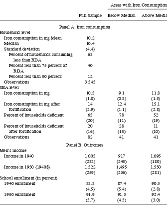
sumption for each household using the number of meals provided by the home. A daily measure of iron intake simplifi es comparisons to the recommended daily al-lowances published by the USDA. Summary statistics are reported in Table 1. Aver-age daily iron consumption for the sample is 10.2 mg with a median of 10.4 mg. Note that the recommended daily allowance for men of working age is 8 mg and for women is 18 mg. About 68 percent of all households in the sample consume less than a household- specifi c RDA determined by the age and gender mix of the household. Because the effects of iron defi ciency are nonlinear, I also report the proportion of the sample that consumes less than 75 percent and 50 percent of the household- specifi c RDA. A surprisingly high proportion of the sample consumes less than these lower cutoffs, 40 percent and 12 percent respectively. Assuming that insuffi cient intake translates to defi ciency, the United States of 1936 experienced similar rates of iron defi ciency as Turkey or Brazil today.
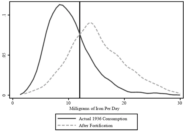
Substantial variation exists across households in the daily consumption of iron. Figure 4 plots the preintervention distribution of household per capita daily consump-tion of iron in the 1936 diets. No similar survey was conducted after the iron fortifi ca-tion program in the 1940s, and so I cannot construct a fi gure by applying the same procedure to later diets. Instead, to see whether the program plausibly affected iron consumption throughout the distribution, I construct an estimated iron distribution by applying the “enriched” iron levels to bread and fl our consumption in the 1936 diets. Figure 4 plots this estimate of the post- intervention distribution for comparison with the original 1936 distribution. Taking diets as given, fortifi cation strongly shifts the distribution to the right, including signifi cant gains for those who were originally at the lower left tail of the distribution. Average consumption of iron increases by 3.8 mg from 10.2 mg to 14 mg, and the proportion of households in the sample predicted to consume less than the recommended daily allowance declines from 68 percent to 23 percent.18 In sum, because store- bought bread and fl our were such common ele-ments in Americans’ diets, it is highly likely that the fortifi cation program signifi cantly boosted iron consumption throughout the distribution.
A later USDA dietary consumption survey from 1955 provides further evidence of the broad impact fortifi cation had on the American diet.19 By at least 1948, nearly all of the white bread purchased by the American public was enriched (Murray et al. 1961). In 1955, survey respondents reported consuming enriched bread products across all regions, income groups, and urbanizations. Table 2 shows that substantial quantities of enriched grain products were consumed in all regions of the country despite concerns about compliance in the South. All areas of the United States were able to, and did, purchase enriched bread.
The fortifi cation program reached those most in need of treatment. Increases in iron consumption occurred along the entire income distribution. In fact, the lower third of the income distribution experienced larger absolute and percentage increases in consumption between the 1936 and 1955 surveys. The counterfactual is stark. Average iron consumption would have been 20 percent less in 1955 without the enrichment
18. The increase in iron consumption here is larger than that using the total U.S. food supply estimates because grain consumption declined by 20 percent from 1936 to 1950. Without this decline in grain consump-tion, the two estimates would be similar.
Table 1
Diet and Outcome Summary Statistics
Areas with Iron Consumption Full Sample Below Median Above Median
Panel A: Iron consumption Household level
Iron consumption in mg Mean 10.2
Median 10.4
Standard deviation (4.4) Percent of households consuming
less than RDA
68 Percent less than 75 percent of
RDA
40 Percent less than 50 percent 12
Observations 3,545
SEA level
Iron consumption in mg 10.5 9.1 11.8
(1.8) (0.8) (1.5)
Iron consumption in mg after fortifi cation
14 12.4 15.1
(2.9) (1.1) (2.8)
Percent of households defi cient 65 78 52
(20) (11) (19)
Percent of households defi cient after fortifi cation
20 28 11
(16) (15) (10)
Observations 82 41 41
Panel B: Outcomes Men’s income
Income in 1940 1,005 917 1,095
(232) (245) (180)
Income in 1950 (1940$) 1,522 1,495 1,550
(259) (236) (281)
School enrollment (in percent)
1940 enrollment 88.8 87.4 90.3
(4.5) (5.4) (2.8)
1950 enrollment 91.9 91.3 92.4
(3.7) (4.3) (3.0)
Sources: Iron consumption and defi ciency come from author’s calculations using “Study of Consumer Purchases, 1935–1936.” See Data Appendix 4 for more detail. Income and school enrollment data provided by census micro-data (IPUMS). Recommended Daily Allowances constructed from Institute of Medicine (2001).
The Journal of Human Resources 922
program. By 1955, 90 percent of households met the RDA for iron and 98 percent of households consumed at least two- thirds of the RDA (Murray et al. 1961).
To facilitate merging with census microdata and to capture the geographic variation in iron consumption before fortifi cation, I calculated the mean daily iron consump-tion over households within each of the 82 SEAs across 30 states. The mean SEA consumes 10.5 mg of iron per person daily with a standard deviation of 1.8 mg. In just under half of the SEAs, the average household consumes less than 10 mg per day. Figure 5 maps the variation across states in the proportion of the sample that consumes less than the household- specifi c recommended daily allowance. The prevalence of defi ciency varies signifi cantly across SEAs and within regions. Signifi cant variation exists within and across census divisions.
Besides iron, enriched bread contained added amounts of niacin and thiamin, in-creasing per capita daily consumption of both vitamins during the early 1940s. Nia-cin, iron, and thiamin consumption are highly correlated at the individual level (ρ = 0.83) and SEA level (ρ = 0.85). Moreover, niacin or thiamin defi ciency essentially implies iron defi ciency. Iron inadequacy is much more prevalent than niacin and thia-min inadequacy in the sample, 68 percent versus 25 and 12 percent. Interpreting the
0
.05
.1
0 10 20 30
Milligrams of Iron Per Day
Actual 1936 Consumption After Fortification
Figure 4
Frequency of Household Iron Consumption in 1936 and Counterfactual Distribution After Fortifi cation
Table 2
Enriched Grain Products Were Consumed by the Entire Population
All
(Non- South) Northeast
North
Central West South
Panel A: Consumption of enriched grain product by region in 1955 (weekly pounds per capita)
Grain products (fl our equivalent)
2.44 2.21 2.59 2.60 3.69
Enriched 1.91 1.72 2.05 2.01 2.50
1936 1955 ∆ in mg percent ∆
Panel B: Iron consumption increased for all income groups
All 11.8 17 5.2 44
Lowest third in income 10.2 16.4 6.2 61
Middle third in income 11.8 17 5.2 44
Highest third in income 14 17.6 3.6 26
Source: Murray et al. (1961).
No Data
0.00–0.56
0.57–0.70
0.71–0.80
0.81–0.90
Figure 5
Percent of State Population Consuming Less than the Recommended Daily Allow-ance in 1936
The Journal of Human Resources 924
reduced- form estimates of the program impact as coming solely from niacin would imply an unreasonable individual effect. Consequently, I focus on iron defi ciency, but at the very least the results can be interpreted as the total effect from reductions in defi ciencies of all three micronutrients.
B. Preexisting Differences in Iron Consumption Are Distributed Quasi- Randomly
The identifi cation strategy relies on the assumption that preexisting geographic dif-ferences in iron consumption across SEAs are not correlated with SEA heterogene-ity in omitted characteristics that induce changes in the outcome. I conduct a direct, albeit partial, test of the identifying assumption by individually regressing SEA aver-age iron consumption on several preprogram SEA characteristics. The assumption is supported if these characteristics do not predict iron consumption, and the exercise suggests specifi c controls if characteristics do have predictive power.20 Point estimates provided in Table 3 suggest that iron consumption is uncorrelated with several eco-nomic, labor market, agricultural, and demographic characteristics. For example, the unemployment rate, New Deal spending, World War II mobilization rates, retail sales and manufacturing output are essentially unrelated to the preexisting differences in iron consumption. Exceptions include per capita war spending, the fraction of the population native born, net migration, and growth in median home values over the 1930s. The results, therefore, suggest adding specifi c controls to the regressions in the following empirical sections. The empirical strategy provides plausibly exogenous variation in health improvements during the 1940s when specifi cations include the additional controls.
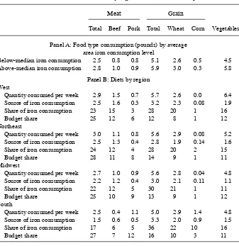
Table 4 explores the proximate cause of geographic differences in iron consumption and variation in the types and quantities of food consumed. Areas with an iron intake below the median of the sample consume less than areas above the median in every food category. However, some of this has to do with geographic differences in tastes for food. In Panel B, diets are broken out by regions of the United States. The South obtains a relatively high proportion of its iron intake from plant- based sources, which are more diffi cult for the body to absorb. The West and Northeast consume a relatively high amount of meat, which has a high absorption rate.
C. Outcome Data
All individual- level outcome data and demographic controls come from the Integrated Public Use Microdata Series (IPUMS, Ruggles et al. 2010), a project that harmonizes decennial census microdata. The basic specifi cation uses census data from 1940 and 1950 as these years bracket the iron fortifi cation program. Income data are limited to 1940 and 1950 as these are the only census years that provide both income and SEA identifi ers. For the school enrollment regressions, additional data from 1910–50 are used to control for gradually evolving SEA specifi c unobserved characteristics. Panel
B of Table 1 contains summary statistics for outcome variables, and the Data Appen-dix 4 provides a more detailed discussion.
V. Forti
fi
cation’s Effects on Contemporaneous Adult
Labor Market Outcomes
In this section, I estimate the changes between 1940 and 1950 in income and labor supply that are associated with increases in iron consumption.21 The census began inquiring about income in 1940, which restricts the analysis to a two- period comparison. However, β can still be identifi ed in regressions that in-clude census- division trends (there are nine census divisions). Table 5 presents point estimates for β, the coeffi cient on (IRONs × POSTt) from Equation 1.22 Because areas with low iron consumption experience larger relative gains, the coeffi cient is expected to be negative if the hypothesis is correct. Standard errors (s.e.) are clus-tered at the SEA- by- year level to allow for a common shock to income at the local level.23
A. Income Gains for Men24
Column 1 provides results from the base specifi cation. The regression includes a census- division time trend as well as individual- level indicators for industry, occupa-tion, veteran status, marital status, race, four educational attainment categories, and an age quartic interacted with education category.25 The point estimate suggests that iron fortifi cation led to statistically and economically signifi cant relative gains in income
21. The full sample includes wage and salary workers aged 18–60 with positive income. I exclude observa-tions without educational attainment information or that are recorded as full- time or part- time students from the income and weeks regressions. Because the 1940 census only inquired about wage and salary income, I exclude observations that list the main class of worker status as self- employed.
22. I choose to use iron consumption to measure the area specifi c intensity of treatment for two reasons: it facilitates the calculation of a reduced- form effect of the program as a whole because we know how much consumption increased following the mandate, and biomedical researchers have recently turned to continu-ous measures of hemoglobin and serum ferritin instead of cutoffs. Response to treatment occurs even if the patient remains below the anemic cutoff, and functional decrements continue after falling below the anemic cutoff (Horton, Alderman, and Rivera 2009). Table A1 reports point estimates for β from Equation 1 using alternative measures of treatment intensity. Differences in the estimated effect compared to Table 5 are negligible.
23. Standard errors are clustered at the SEA by year level according to the procedure developed by Liang and Zeger (1986). Correlation of unobserved shocks to individuals within the same SEA in the same year is the main concern. Serial correlation does not pose a serious problem as the time periods in the panel are separated by ten years (Bertrand, Dufl o, and Mullainathan 2004). In the full sample, the number of clusters = 164. Results from regressions that aggregate to the SEA level using the procedure developed by Donald and Lang (2007) are consistent with those of the microdata regressions.
24. I split the analysis by sex based on the radically different labor market incentives facing men and women during the 1940s. I focus the analysis on men in the main text because the sample sizes for working women are small. In general, unmarried women behave as if fortifi cation had positive effects on productivity, but married women do not. The appendix contains a more detailed analysis of the labor market impacts for women.
The Journal of Human Resources
926
Table 3
State Economic Area Predictors of Average Iron Consumption
Economic and labor
market conditions Migration Retail sales
War spending per capita
Unemployment rate
Average income (1936)
Net migration (1930–40)
Retail sales per capita (1939)
Retail sales growth (1929–39)
Point estimate –0.16* 21.6 0.046 0.037* 0.095 –0.36
Standard error (0.09) (24.3) (0.047) (0.020) (0.075) (2.14)
R2 0.02 0.01 0.02 0.03 0.02 0.000
Fraction of population (1940) Manufacturing (1940)
Native born Black Urban Average wage
Output per capita
Value added per worker
Point estimate –5.63* –0.011 –0.04 0.001 0.0003 0.0004
Standard error (3.20) (0.011) (0.07) (0.008) (0.0009) (0.002)
R2 0.038 0.012 0.003 0.000 0.001 0.001
Housing (1940)
Percent homeowner
Median home value ($1,000)
Percent
∆median home
value (1930–40)
Percent with electricity
Percent with radio
Percent with refrigerator
Point estimate 0.008 –0.125 –2.96* 0.003 0.003 0.001
Standard error (0.016) (0.238) (1.62) (0.009) (0.008) (0.014)
Niemesh
927
Crop value per acre
Farm value
per acre Fraction tenant
Dustbowl county
Average
temperature Average rainfall
Point estimate 0.02 0.003 –0.99 –1.0 0.003 –0.11
Standard error (0.013) (0.002) (0.91) (2.5) (0.031) (0.17)
R2 0.024 0.027 0.01 0.002 0.001 0.005
New Deal spending ($1,000) WWII mobilization
Total grants per capita
Relief grants per capita
Public work grants per capita
Loans per
capita SEA mobilization rate
Point estimate 1.4 7.1 –0.5 0.20 0.45
Standard error (3.7) (4.3) (3.9) (0.25) (2.2)
R2 0.003 0.026 0.000 0.01 0.000
Sources: New Deal spending, retail sales, weather and migration data were compiled for Fishback, Kantor, and Wallis (2003) and Fishback, Horrace, and Kantor (2005, 2006). Copies of the data sets can be obtained at the following website: http: // www.u.arizona.edu / ~fi shback / Published_Research_Datasets.html. Income is from the “Study of Con-sumer Purchases.” World War II mobilization rates constructed by author using enlistment data from the Selective Service System and population counts of 18–64- year- old males from IPUMS. All other data is from Haines and ISPCR (2010).
The Journal of Human Resources 928
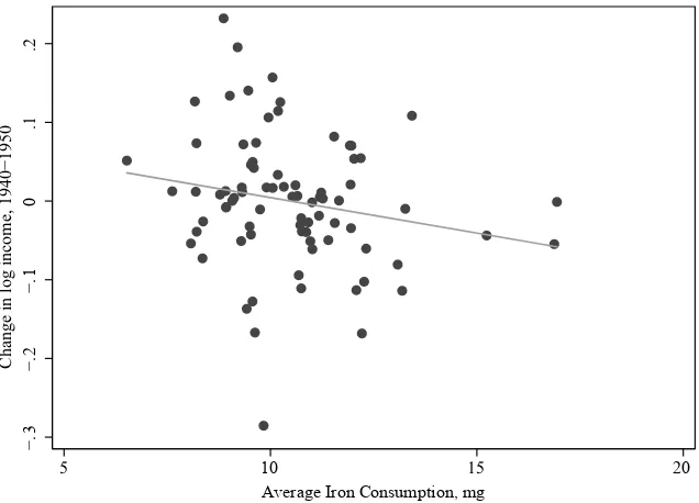
over the 1940s for men in areas with lower iron consumption, which is graphically represented in Figure 6. The result is robust to regional convergence in wages over the decade.
For a public health program that was relatively inexpensive at 0.50 dollars per capita annually (Wilder and Williams 1944), the economic impact on wage income alone is impressive. The base estimate for men suggests a one standard deviation
dif-Table 4
Variation in Diets as the Proximate Cause of Differences in Iron Consumption
Meat Grain
Total Beef Pork Total Wheat Corn Vegetables
Panel A: Food type consumption (pounds) by average area iron consumption level
Below- median iron consumption 2.5 0.8 0.8 5.1 2.6 0.5 4.5 Above- median iron consumption 2.8 1.0 0.9 5.9 3.0 0.3 5.8
Panel B: Diets by region West
Quantity consumed per week 2.9 1.5 0.7 5.7 2.6 0.0 6.4 Source of iron consumption 2.5 1.6 0.3 3.2 2.3 0.08 1.9
Share of iron consumption 23 15 3 28 20 1 16
Budget share 25 12 6 12 8 1 12
Northeast
Quantity consumed per week 3.0 1.1 0.8 5.6 2.9 0.08 5.2 Source of iron consumption 2.5 1.3 0.4 2.8 1.9 0.14 1.6
Share of iron consumption 24 12 4 28 20 2 15
Budget share 28 11 8 14 9 1 11
Midwest
Quantity consumed per week 2.7 1.0 0.9 5.6 2.8 0.04 4.8 Source of iron consumption 2.2 1.2 0.4 3.0 2.1 0.11 1.1
Share of iron consumption 22 12 5 30 21 1 11
Budget share 25 10 9 13 9 1 12
South
Quantity consumed per week 2.5 0.4 1.1 5.0 2.9 1.4 4.8 Source of iron consumption 1.5 0.6 0.5 3.3 2.0 0.9 1.5
Share of iron consumption 17 6 5 36 22 10 16
Budget share 27 7 12 16 10 3 11
Sources: Author’s calculations using “Study of Consumer Purchases, 1935–1936” and USDA (2009).
ference (1.8 mg) in SEA average iron consumption was associated with a 2.6 percent difference in income growth.
Besides iron, enriched bread contained added amounts of niacin and thiamin, in-creasing per capita daily consumption of both vitamins during the early 1940s. An attempt to tease out the impact of each micronutrient individually was inconclusive.26 At the very least, the results can be interpreted as the reduced form total effect from bread fortifi cation.
Robustness Checks
Potential threats to a causal interpretation of β remain in the form of unobserved SEA- specifi c shocks to income that are correlated with iron consumption. For example,
26. Less than 1 percent of observations that are thiamin defi cient and less than 5 percent of observations that are niacin defi cient are not also defi cient in iron. High collinearity notwithstanding, I regress income and school enrollment on niacin, thiamin, and iron consumption individually and combined. When included separately, the reduced form results are all similar due to the high levels of correlation between the measures. When included together, the results are inconclusive. For the specifi cation including all three measures, the point estimates and standard errors are –0.015 (0.010) for iron, –0.003 (0.004) for niacin, and –0.005 (0.038) for thiamin from the income regression.
í
3
í
2
í
1
0
&KDQJHLQORJLQFRPHí
10 20
Average Iron Consumption, mg
Figure 6
Areas with Low Initial Iron Consumption Experienced Larger Gains in Male Income
The Journal of Human Resources
930
Table 5
Results for Contemporaneous Adult Male Labor Market Outcomes
Log Wage and Salary Income (Percent) Labor Force Participation (p.p.) Conditional Weeks (Per Year)
1 2 3 4 5 6 7 8 9 10
Iron consumption (mg) –1.44*** –1.05** –0.92** –1.04* 0.17 0.10 0.06 –0.15* –0.16** –0.09
(0.46) (0.42) (0.46) (0.57) (0.16) (0.14) (0.15) (0.09) (0.08) (0.08)
Individual level controls
Nonwhite –30.3*** –30.2*** –24.3*** –49.5*** –2.50*** –2.52*** –3.79*** –1.6*** –1.5*** –1.6***
(1.9) (1.9) (2.4) (2.7) (0.58) (0.58) (0.56) (0.25) (0.25) (0.29)
Married 28.4*** 28.4*** 29.0*** 35.9*** 6.02*** 6.02*** 5.95*** 3.2*** 3.2*** 3.2***
(0.6) (0.6) (0.6) (0.8) (0.48) (0.48) (0.50) (0.22) (0.22) (0.24)
Veteran 0.55 0.57 0.44 3.97*** –1.94*** –1.95*** –1.77*** 0.21 0.21 0.28*
(0.90) (0.90) (0.92) (1.11) (0.52) (0.52) (0.53) (0.17) (0.17) (0.17)
Veteran of WWII –1.94 –1.92 –2.25 –4.88*** 1.09* 1.07* 0.88 –0.70** –0.70** –0.83***
(1.47) (1.48) (1.42) (1.60) (0.60) (0.60) (0.60) (0.30) (0.30) (0.30)
Occupation indicator YES YES YES NO NO NO NO NO NO NO
Industry indicator Quartic in age x
YES YES YES NO NO NO NO NO NO NO
Education level YES YES YES YES YES YES YES YES YES YES
SEA level controls (interacted with POSTt) WWII mobilization
rate (p.p)
0.10 0.15 0.007 –0.83 –2.61 0.01 –0.02
(0.09) (0.11) (0.11) (2.67) (3.15) (0.01) (0.02)
Unemployment rate (p.p.)
–4.14*** –4.38*** –5.72*** 2.61 4.59 –0.69*** –0.61***
Niemesh
931
Preintervention income ($100)
0.19* 0.21* 0.20 0.048 0.068 0.05** 0.07**
(0.11) (0.12) (0.14) (0.060) (0.063) (0.02) (0.03)
Net migration (p.p. 1940–50)
–5.0 –4.9 –10.4* –0.27 –0.668 –0.02* –0.03***
(5.4) (5.9) (6.1) (1.66) (1.87) (0.009) (0.008)
New Deal expenditures ($100 per capita)
0.63 1.18 0.66 –0.41 0.16 0.35 0.57**
(1.33) (1.48) (1.65) (0.51) (0.47) (0.24) (0.25)
House price growth (percent 1940–50)
–6.9 –5.6 –1.3 –0.71 0.68 –2.1* –0.27
(5.9) (6.4) (7.2) (1.50) (1.93) (1.2) (1.3)
Census division time trend YES YES YES YES YES YES YES YES YES YES
SEA fi xed effect YES YES YES YES YES YES YES YES YES YES
Observations 116,486 116,486 108,324 116,993 158,921 158,921 144,278 116,762 116,762 108,565
R- squared 0.520 0.520 0.494 0.439 0.047 0.047 0.048 0.092 0.092 0.093
Sources: Individual outcomes and controls come from IPUMS. Unemployment, war spending, and house prices are from Haines and ISPCR (2010). New Deal spending and migration data were compiled for Fishback, Kantor, and Wallis (2003) and Fishback, Horrace, and Kantor (2005, 2006). SEA average iron consumption and income are calcu-lated by the author from the “Study of Consumer Purchases.”
The Journal of Human Resources 932
heterogeneity in local labor market conditions due to wartime spending and mean reversion from the depths of the Great Depression (perhaps) could be correlated with iron consumption in the 1930s. Similarly, a temporary negative shock might simulta-neously cause low iron consumption and low income in 1936. As the temporary shock dissipates, we would expect income gains correlated with low iron consumption even if fortifi cation had no effect. Moreover, the wartime economy made a long- lasting impact on female labor force participation and male wages (Acemoglu, Autor, and Lyle 2004). To reduce the scope for such omitted variable bias, Column 2 of Table 5 includes the SEA- level WWII mobilization rate, 1937 SEA- level unemployment rate, 1936 SEA average income, per capita World War II spending, total New Deal expen-ditures, net migration over the 1940s, and median house price growth, all interacted with POSTt. The results are little changed, suggesting that conditional on the control variables, geographic differences in preprogram iron consumption are uncorrelated with omitted heterogeneity causing income gains.27 Using the estimate from Column 2 with the full set of controls, a one- milligram difference in average iron consumption is associated with a 1.05 percent difference in wage and salary income growth. Increas-ing SEA average iron consumption by 2 mg translates into a 2.1 percent increase in income between 1939 and 1949.28 For perspective, this would account for close to 4 percent of the total income growth over the decade in the areas below the median of iron consumption.
A number of public health programs were conducted in the Southern states simul-taneously with the bread enrichment program. Hookworm and malaria eradication efforts continued into the 1940s in parts of the South. Moreover, some Southern states allowed for voluntary enrichment of bread and fl our with B vitamins starting in 1938. Surveys, however, indicated Southern bakers and millers did not participate in the voluntary programs (Wilder and Williams 1944). Column 3 drops the Southern states from the sample to limit identifi cation of the effects of iron fortifi cation to variation from states in the Northeast, Midwest, and West census regions. Dropping the South has little effect on the point estimate.
The choice of industry and occupation may be endogenous to a change in health caused by increased iron consumption. For example, a worker might upgrade to a higher- paying occupation or industry because of increased endurance or work capac-ity. The coeffi cient estimates from regressions without controls for occupation and industry are essentially unchanged from before, as reported in Column 4. Thus, the relative gains in income do not appear to be caused by occupational upgrading. A re-gression using the IPUMS occscore variable as the dependent variable gives a similar interpretation (results unreported).
American diets underwent substantial changes during the 1940s in response to ra-tioning and a large demand for food on the part of the U.S. military and allies. These
27. Point estimates are similar when limiting the sample to native- born or foreign- born men. Cross- state migration does not explain the results. Regressions limiting the sample to native- born men residing in their state of birth provide identical point estimates to those in Column 2. Point estimates from adding the SEA Gini coeffi cient for male wage and salary income suggests that the income gains correlated with low iron consumption are not explained by a compression of wages during the 1940s. However, this measure captures within- SEA compression of the wage distribution but not wage compression across SEAs.
changes, however, were not long lasting. Diets returned to their prewar patterns shortly after rationing was discontinued in 1946. While fl uctuations in the consumption of nonenrichment nutrients briefl y improved overall nutritional status, they do not ap-pear to drive the empirical results I fi nd in this section. The appendix provides evi-dence from the medical literature, the diet survey data, and regressions that include other micronutrients as explanatory variables. Rationing of foodstuffs during the war potentially improved diets by reducing the inequality in consumption of iron. The results are essentially unchanged when an SEA Gini- coeffi cient of iron consumption is included as a control. Moreover, I fi nd no statistically signifi cant effect of inequality of iron consumption when the Gini replaces average iron consumption as the variable of interest.29
B. Labor Supply of Men
The above regressions clearly point to relative gains in income over the 1940s cor-related with low preprogram iron consumption for young male workers. Iron fortifi ca-tion may have promoted these gains through a number of potential channels: labor supply could change at the intensive or extensive margins, or productivity per unit of time could rise. All three channels may have worked simultaneously but not necessar-ily in accordance with each other. I attempt to shed light on these issues by conducting separate regression analyses for labor force participation, weeks worked, and hours worked.
Columns 5–10 of Table 5 offer a direct assessment of the labor supply channels. La-bor force participation by men in 1940 was already quite high and had little room for improvement. Thus, it is no surprise that only small changes on the extensive margin of work were associated with preintervention iron consumption. The results are gener-ally consistent with small relative decreases in male labor force participation rates in areas with low iron consumption. However, the estimates are imprecise. Adjustments along the extensive margin do not seem prevalent and are unlikely to drive the income results of Table 5.
Changes at the intensive margin are explored using the weekly hours and weeks worked variables. Conditional on working positive hours, changes in weekly hours are not correlated with preintervention iron consumption (results unreported). Columns 8–10 of Table 5 report point estimates from regressions with a continuous measure of weeks worked as the dependent variable. The results are broadly consistent with rela-tive increases in weeks worked correlated with low preintervention iron consumption, although the estimates are noisy. The point estimate with full controls corresponds to an increase of three- quarters of a day of work or 0.4 percent of the 1940 mean. Evaluated at the mean of weeks worked in 1940 (44) for the full sample and for a one- milligram increase in iron consumption, gains on the intensive margin of labor supply account for just over one- third of the total increase in income. In general, it appears that men responded to reductions in iron defi ciency by adjusting labor supply along the intensive margin. However, changes in hours and weeks worked do not explain the full effect of iron fortifi cation on income.
The Journal of Human Resources 934
C. Interpretation of Men’s Labor Market Results
As an external check to the validity, I compare the results to those found in the devel-opment and medical literatures, which report average treatment effects on the treated for patients preidentifi ed as anemic or iron defi cient. My results pertain to an ag-gregate level effect on the total population, not solely anemic patients.30 I convert the average aggregate result to a parameter similar to an “average treatment effect on the treated” or “an intent to treat effect“ for an iron defi cient individual.
The fortifi cation program differentially affected individuals, with larger benefi ts accruing to those with lower initial levels of iron. I assume that only those individuals consuming less than 75 percent of their RDA experienced gains in health from the program and thus gains in income. Concentrating the full reduced- form impact of the program onto this portion of the population gives the average income gain to the iron- defi cient individual. Using the results from Column 2 of Table 5, a difference of one mg in preintervention iron consumption implies a differential 1.05 percent gain in income. On average, the program increased iron consumption by 2 mg per day (Gerrior, Bente, and Hiza 2004). Therefore, the full reduced- form effect on income of the program was 2.1 percent. Dividing by the proportion of the sample that con-sumed less than 75 percent of the RDA suggests that the program increased incomes by 5.25 percent at the individual level. Applying this procedure to labor supply sug-gests that the program increased weeks worked by 1.82 percent at the individual level. The remainder, 3.43 percent, can be interpreted as the productivity effect (wage / hour). A major contribution of this paper is the result that increased labor supply makes up a large portion of the total increase in income associated with the iron fortifi cation program. Estimated benefi t- cost ratios that rely solely on the productivity impacts will underestimate the true benefi ts of an iron fortifi cation campaign.
The result for the individual productivity effect is well within the range of values found in fi eld experiments in the developing country context. Thomas et al. (2006) fi nd a 30 percent increase in productivity for preidentifi ed anemic self- employed In-donesian males in a randomized study of iron supplementation. Rubber tappers in Indonesia were found to have increased productivity by 10–15 percent (Basta et al. 1979). Chinese textile workers increased production effi ciency by 5 percent after supplementation (Li et al. 1994), and Sri Lankan tea pickers increased the amount of tea picked by 1.2 percent (Edgerton et al. 1979).
VI. Iron Forti
fi
cation’s Contemporaneous
Effects on School Enrollment
In this section, I estimate the gains in school enrollment associated with increases in iron consumption. The census asked about school enrollment well before 1940, which allows me to extend the analysis from the two- period case in the previous section. First, I document the advantage in school enrollment experienced by
areas with high levels of iron consumption and the abrupt decline of consumption in the 1940s. Second, focusing on the 1940–50 period, I estimate a two- period specifi ca-tion similar to those discussed in the previous secca-tion. Finally, I extend the sample to the early 20th century to allow estimation with location- specifi c time trends, which are the preferred estimates for the causal impact of the fortifi cation program.
Using the fi ve decades of census data, I explore the timing of the relationship between changes in school enrollment and iron consumption. Figure 7 plots the es-timated coeffi cient on IRONs from regressions using each year of census data as a separate sample. The correlation between iron consumption and school enrollment is stable and positive during the decades prior to the enrichment program. Prior to the introduction of enriched bread, areas consuming more iron in their diet have higher enrollment rates. Only during the 1940s does the relationship make a sharp decline. Consequently, the timing of relative gains in school enrollment for low iron consump-tion SEAs coincides with the federal fortifi cation mandate. I now turn to estimating the reduced form causal impact of the fortifi cation program on school enrollment.
Enrollment is measured as a binary indicator equal to one if the child attended school for at least one day during the census reference period. Table 6 presents point estimates for β, the coeffi cient on (IRONs × POSTt). Each entry is from a separate estimation of Equation 1, with the full sample limited to children aged 8–17. Again, because areas with lower iron consumption before fortifi cation are hypothesized to have experienced larger improvements in health after fortifi cation, the coeffi cient is expected to be negative if the hypothesis is correct. Standard errors are clustered at the SEA- by- year level. Regressions control for race, sex, and race and sex interacted with POSTt, and age dummies, at the individual level. Year and state economic area indicators are also included.
Column 1 of Table 6 reports point estimates for β from the base specifi cation of Equation 1 for the full sample of children aged 8–17 spanning 1940–50. Results are consistent with the hypothesis that fortifi cation led to greater schooling. A one mg difference in iron consumption is associated with a 0.47 percentage point differential change in school enrollment rates. As a placebo test, I estimate the two- period specifi -cation of Equation 1 separately for the 1910–20, 1920–30, and 1930–40 samples. As expected, changes in school enrollment are not correlated with 1936 iron consumption in any of the prior decades when no major changes in iron consumption occurred.31 Again, the timing of schooling gains in low iron consumption areas coincides with the fortifi cation program.
Potential threats to a causal interpretation of β remain in the form of unobserved area specifi c shocks to or trends in enrollment correlated with iron consumption. For example, regional convergence in school enrollment rates could confound the estimate to the extent that low enrollment areas also tended to be low iron areas. The wealth of data contained in the IPUMS allows me to extend the sample to include the 1910–50 censuses and, therefore, SEA- specifi c time trends (Column 2) and census- division time trends (Column 3).32 Identifi cation of β now comes from deviations of
enroll-31. Estimates by sample year: 1910–20: β = 0.0003(0.003); 1920–30: β = –0.0009(0.003); 1930–40: β = 0.0016(0.002).
The Journal of Human Resources 936
ment during the 1940s from the preexisting geographic trend. The point estimates are larger in magnitude than those without controlling for a trend.33 The preferred estimates are those in Column 3 that include the census division trend as these tend to be more conservative than results from including an SEA- specifi c trend. Using the preferred estimates, the impact of iron fortifi cation on school enrollment is economi-cally signifi cant—a one standard deviation difference in iron consumption implies a difference in school enrollment of one percentage point.34
It is also possible that differential changes in parental income and education were correlated with the measure of iron consumption and therefore could confound in-terpretation of β. The time trends should control for this to some extent, but, ide-ally, individual- level controls for parental education and income could be included. Unfortunately, the sampling procedures for the 1950 census instructed that detailed sample- line questions were to be asked of a single member of the household. School
33. Results are robust to clustering at the level of the state economic area to allow for arbitrary serial cor-relation of the error terms.
34. Iron drives the impact on school enrollment from enriched bread, not niacin or thiamin. For the specifi ca-tion including all three measures, the point estimates and standard errors are –0.7 (0.3) for iron, 0.08 (0.2) for niacin, and 0.016 (0.016) for thiamin.
í
5
0
1
5
1910 1920 1930 1940 1950
Beta 95% CI
Figure 7
Timing of School Enrollment Gains Coincides with Enrichment Program
enrollment and income variables are never recorded together within the same respon-dent household. Therefore, I use average SEA measures of income and education as an alternative strategy. I calculate average real wage and salary income for males and the proportion of the population that has completed high school, some college, or college for each SEA in 1940 and 1950 using individuals between the ages of 25 and 50. As seen in Column 4 of Table 6, the inclusion of parental controls reduces the magnitude of the point estimates. However, the results are still consistent with iron fortifi cation having a positive impact on school enrollment rates. Moreover, parental income is a potentially endogenous control, and one could argue that it should be excluded. As such, Column 4 may be interpreted as decomposing the full effect of iron fortifi cation on enrollment into its “direct” effect and the portion from fortifi cation’s effect on parental income.
The effects of fortifi cation do not seem to be concentrated in one single demographic group, although there are some important differences. Theory suggests that groups closer to the margin of school enrollment experience larger effects from iron fortifi -cation. Columns 5–8 of Table 6 report point estimates for β from regressions using distinct demographic subsamples. The percentage point increase for 13–17- year- olds is roughly twice that of the 8–12- year- olds, however, the estimates are noisy for the older group. School enrollment of the younger age group was already quite high in 1940 at 96 percent whereas it was only 82 percent for the older age group. The es-timated effect for nonwhites is over three times that of whites. Overall, the results suggest a slightly larger effect for demographic subgroups that on average are closer to the margin of attending school.
As a fi nal robustness check, Column 9 drops the South census region from the sample. The point estimates are smaller and lose statistical signifi cance. However, specifi cations using the 1940–50 periods, with and without limiting to within- region variation, and the full SEA time- trend all have economically large and statistically signifi cant point estimates.35 As such, the impact of iron fortifi cation on schooling gains should be interpreted with the caveat that public health programs and the overall regional gains in school enrollment in the South over the early 20th century might potentially drive the result.
VII. Long- Term Effects on Children
The impact of iron defi ciency during infancy and early childhood might extend to long- term effects manifested during adulthood. I follow up on chil-dren that potentially benefi tted from the iron fortifi cation mandate by looking at their corresponding adult outcomes using the 1970 decennial census microdata. Economic outcomes I examine include income, years of schooling, and poverty status as an adult. The cross- cohort comparison comes from older cohorts having less time to gain during childhood from the fortifi cation program. Similarly, children born in states with high preexisting iron consumption also had less scope for improvements.