Why Are the Returns to Schooling
Higher for Women than for Men?
Christopher Dougherty
A B S T R A C T
Many studies have found that the impact of schooling on earnings is greater for females than for males, despite the fact that females tend to earn less, both absolutely and controlling for personal characteristics. This study investigates possible reasons for this effect, using data from the National Longitudinal Survey of Youth 1979–. One explanation is that education appears to have a double effect on the earnings of women. It increases their skills and productivity, as it does with men, and in addition it appears to reduce the gap in male and female earnings attributable to factors such as discrimination, tastes, and circumstances. The latter appear to account for about half of the differential in the returns to schooling.
I. Introduction
Differentials in earnings by sex and ethnicity, persistent despite legis-lation against discrimination, have provoked a large and growing investigative litera-ture (for surveys, see Lloyd and Neimi 1979; Treiman and Hartmann 1981; Madden 1985; Cain 1986; Gunderson 1989; Blau and Kahn 1992; Altonji and Blank 1999; Blau and Kahn 2000). The standard approach to the analysis of the determinants of earnings differentials, the Blinder-Oaxaca decomposition, involves the fitting of a Mincerian semilogarithmic wage equation
(1) lnY iXi u
i k
0 1
=b + b +
=
!
where Yis a measure of earnings, the Xiare a set of k personal and labor market
characteristics, and uis a disturbance term. In the case of sex differentials, the func-tion is fitted for male and female samples separately. Using superscripts mand ffor
Christopher Dougherty is a senior lecturer in economics at the London School of Economics. He wishes to thank colleagues at the LSE Centre for Economic Performance and three anonymous referees for helpful comments. The data used in this article can be obtained beginning May 2006 through April 2009 from the author, <c.dougherty@lse.ac.uk>.
[Submitted August 2003; accepted February 2005]
ISSN 022-166X E-ISSN 1548-8004 © 2005 by the Board of Regents of the University of Wisconsin System
males and females, and noting that the fitted equations pass through the sample
Subtracting Equation 3 from Equation 2, the difference can be written
(4) lnYm lnYf i(X X ) ( ) X ( )
(Blinder 1973; Oaxaca 1973). The first term is said to measure that part of the earn-ings gap attributable to male-female differences in the characteristics and the other two that part attributable to differences in the wage effects of the characteristics.1 Usually the wage-effect part is attributed to discrimination, but this can be somewhat misleading, for it may be argued that some of the differences in the coefficients may reflect the influences of other factors. In particular, some women may have tastes for certain kinds of work that cause them to be concentrated in relatively poorly paid occupations.2For others, circumstances may be a factor. In particular, women with children may rationally be willing to accept a wage offer that undervalues their char-acteristics if the job fits well with other responsibilities. In acknowledgment, the male-female difference in mean wages attributable to differences in coefficients will here be attributed to discrimination, tastes, and circumstances (DTC).
In the case of the United States, where the difference in earnings has been dimin-ishing (O’Neill and Polachek 1993; Blau and Kahn 2000), the component attributa-ble to differences in characteristics is now considered to be relatively small. Accordingly interest has become focused on the DTC component. Some authors, fol-lowing the example of Blinder (1973), have attempted to divide this part of the gap into subcomponents attributable to differences in the coefficients of individual char-acteristics and to the difference in the intercepts (“pure discrimination”), but such a decomposition is illegitimate (Jones 1983; Oaxaca and Ransom 1999).3 Nevertheless, the signs of the differences in the coefficients are of interest and, given that the DTC component favors males, one might expect that for the two most impor-tant variables, schooling and work experience, the female coefficients will be smaller. While this appears to be the case for work experience, it surprisingly does not appear to be true for schooling. Indeed, if anything, there appears to be a tendency for the estimated schooling coefficient to be largerfor females.
II. Previous Findings
Although the studies that have investigated male and female earnings are now legion, the number that actually report separate schooling coefficients is much smaller. Many of those focusing on the returns to education4with data on both sexes have fitted pooled regressions, allowing for a sex differential by including a sim-ple dummy variable with no interactive term. Where separate regressions have been run, schooling is often among the unreported controls. In the case of the subliterature on the earnings gap, the single most plentiful source of studies with separate regres-sions, the regression coefficients are sometimes not reported at all.
Appendix 1 summarizes the 27 U.S. studies that satisfy three conditions:
(1) the study reports either male and female schooling coefficients in parallel regressions, or a joint regression that includes a female-schooling interactive term;
(2) a Mincerian semilogarithmic specification is used for the wage equation;
(3) the controls do not include either occupation or industry, and the sample is not restricted narrowly by occupation or industry.
The list is intended to be comprehensive, though doubtless some eligible studies have been missed.
The second condition occurs because it is generally impossible to derive compara-ble schooling coefficients from studies that have used a linear specification for earn-ings and so a number of widely cited studies (Cohen 1971; Suter and Miller 1973; Featherman and Hauser 1976; Roos 1981; Grubb 1993) have had to be discarded. The linear model is in any case a misspecification (Heckman and Polachek 1974; Dougherty and Jimenez 1991).
The reason for the third is that much of the impact of schooling on earnings is medi-ated by occupational attainment and, perhaps to a lesser extent, by industrial recruitment. Accordingly the use of occupational and/or industrial controls, popular in the male-female earnings gap literature as a means of assessing how much of the gap is attributa-ble to occupational segregation, strips the schooling control of much of its impact.
As can be seen from Appendix 1, most of the studies have used data from large, nationally representative data bases: the National Longitudinal Studies of Labor Market Experience, the Panel Study of Income Dynamics, the Current Population Survey, Censuses of Population, and the National Longitudinal Study of the High School Class of 1972 and its successor, High School and Beyond. Most of them have used years of schooling as the educational variable but some have used sets of dummy variables. The latter approach makes male-female comparisons of the returns to schooling less straightforward, but in some cases it does provide an opportunity for attempting to identify the schooling level at which the returns diverge. Most of the studies have used actual work experience and its square as controls. However some
4. By this is meant the proportional increase in earnings per year of schooling, following conventional usage. The expression is not intended to refer to the Fisherian internal rate of return. See Psacharopoulos (1981) for a discussion of the conditions under which the schooling coefficient might be interpreted as an approximation to the internal rate of return.
have used potential work experience and three have used age as a proxy. They vary widely in their use of other controls.
Of the 27 studies, 18 report unambiguously higher schooling coefficients for females. Six report multiple estimates where the female coefficients are mostly higher.5Two report mixed results that are evenly balanced.6Only one reports higher schooling coefficients for males, and this study had a relatively small sample.7In gen-eral the studies report only point estimates, and it is thus impossible to determine whether the differences in the coefficients are significant. However, taking the studies together, the effect is undoubtedly significant, for under the null hypothesis that the coefficients are the same; the probability of 24 out of 27 studies finding higher coef-ficients for either sex is less than 0.01 percent.
As to which levels of schooling are responsible for the effect, there is some evi-dence that the returns to partial and complete college are higher for females than for males; for years of high school, the evidence points the other way; and for postgrad-uate studies, the evidence is mixed.8
Given the institutional differences between the labor market in the United States and labor markets in other countries, one would not anticipate that a feature of the U.S. mar-ket would necessarily be encountered elsewhere. However, two recent surveys suggest that the effect may not be confined to the United States. Trostel, Walker, and Woolley (2002) estimate the returns to schooling in 28, mostly European, countries with data derived from a common survey instrument and found that the female schooling coeffi-cient was higher in 24. Psacharopoulos and Patrinos (2002) list 95 estimates of male and female schooling coefficients from 49 countries at different dates. Of these 63 are greater for females, three are equal, and 23 are greater for males.
III. Possible Causes of the Effect
Candidates for an explanation of the male-female differential in the schooling coefficient include the following possibilities: an inverse relationship between
5. Angle and Wissman (1981), Gregory et al. (1989), Blau and Kahn (1997), and Brown and Corcoran (1997) use dummy variables for education and thus have different estimates for different levels. Gwartney and Long (1978) and Carlson and Swartz (1988) have multiple estimates because they fit wage equations for nine and 12 ethnic categories, respectively. In each of these studies most of the estimates of the returns to schooling are higher for females.
6. Kane and Rouse (1995) find higher returns to schooling for females using the NLS72 data but mostly lower ones using NLSY data. Mincer and Polachek (1974) find that males have higher returns than married females but lower ones than single females.
7. Barron, Black, and Lowenstein (1993).
years of schooling and DTC; a male-female differential in the quality of educational attainment; occupational segregation of females into sectors where the returns to school-ing are relatively high; biased estimates attributable to a failure to take account of sam-ple selection; and biased estimates attributable to a failure to take account of the endogeneity of schooling or work experience. Doubtless this list is incomplete.
The present intention is to argue that, of these explanations, the first may be an important one. It is suggested that schooling may have two effects on earnings, at least for females: a direct human capital effect, and an indirect effect via an attenuation of the adverse impact of DTC.
There are two reasons for hypothesizing that the impact of discrimination may not be uniform in the labor market and that, in particular, it may be inversely related to the level of schooling. First, it is possible that the better educated an individual is, the more likely he or she is to have a degree or other formal qualification that would help to standardize wage offers regardless of sex. Second, it is possible that the better edu-cated a woman is, the more likely she is to be capable of resisting discrimination. Similar arguments may be made with respect to that component of the unexplained earnings gap attributable to tastes and circumstances. It is possible that the better edu-cated a woman is, the more likely she is to be willing to seek employment outside the low-paying traditionally female occupations. At the same time, it is possible that the better educated she is and the greater her potential earnings, the more capable she is of paying for childcare and other services that allow her to seek a wage offer that fully values her characteristics. The impact of these factors may be inversely related to the level of schooling and failure to allow for them could impart an upward bias in the estimated female schooling coefficient.
IV. Evidence from the National Longitudinal Survey
of Youth 1979–
A. Data and Method
The data set used for the present analysis is the NLSY 1979–, a panel study sponsored by the Bureau of Labor Statistics and managed by the Center for Human Resource Research at the Ohio State University. It consists of a nationally representative core sample of 6,111 individuals aged 14–21 in 1979, the base year, and supplementary oversamples of minorities, poor whites, and those serving in the military. The survey was fielded annually until 1994 and since then it has been fielded biennially.
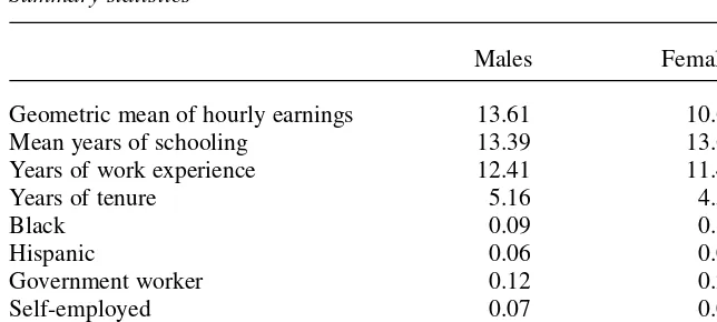
The data used in the present analysis were taken from the core sample, the hourly earnings and other work variables as pooled data for the current or most recent job at the 1988, 1992, 1996, and 2000 interviews, with earnings being converted into 1996 constant dollars using the Urban Consumer Price Index. For the wage equations observations were dropped if the respondent was currently attending school, if high school transcript data had not been collected or were incomplete, if hourly earnings were less than $2.50 or more than $100 at 1996 prices, if hours worked were 0 or exceeded 60, or if there were missing data. Altogether in the wage equations there were 11,451 observations relating to 3,852 individuals. Table 1 presents summary statistics for key variables.
To take account of the fact that there were multiple observations for most respon-dents, the model was fitted using random effects, the appropriate procedure in the case of a random sample from a large population if the unobserved heterogeneity is inde-pendent of the correlates (Baltagi 2001; Hsiao 2002). One attraction of the NLSY data set for fitting wage equations is that it includes a large number of control variables including, in particular, measures of cognitive ability that allow one to minimize potential bias attributable to unobserved heterogeneity. Fixed effects estimation would in principle have been preferable, but the schooling variable would have been washed out.9
B. Results
Column 1 of Table 2 shows the result of a conventional regression of the logarithm of hourly earnings on a female dummy variable, years of schooling, and a set of control variables. The latter comprised actual work experience and its square; tenure with the current employer and its square; dummy variables for black and Hispanic ethnicity; a dummy variable for being married with spouse present; the arithmetic reasoning, word knowledge, paragraph comprehension, numerical oper-ations, and coding speed test scores from the Armed Services Vocational Aptitude Battery; dummy variables for living in the country or on a farm when aged 14; a dummy variable for the purchase of magazines by anyone in the family when the respondent was aged 14; a dummy variable for living in the northeast, north-central, or west census regions; a dummy variable for living in an urban area; and the local unemployment rate. All of the control variables were interacted with the female dummy variable.
9. A Hausman test rejects random effects in favor of fixed effects, but this is inevitable with such a large sample.
Table 1
Summary statistics
Males Females
Geometric mean of hourly earnings 13.61 10.63 Mean years of schooling 13.39 13.63 Years of work experience 12.41 11.45 Years of tenure 5.16 4.54
Black 0.09 0.11
Hispanic 0.06 0.07
Government worker 0.12 0.20
Self-employed 0.07 0.05
Dougherty
975
Table 2
Wage equations, dependent variable logarithm of hourly earnings
(1) (2) (3) (4) (5)
Female −0.3560** −0.3917** −0.1636 −0.1232 0.0958
(0.0968) (0.0976) (0.1076) (0.1112) (0.1307)
Schooling 0.0490** 0.0491** 0.0505** 0.0490** 0.0505**
(0.0041) (0.0041) (0.0046) (0.0041) (0.0046)
Schooling* female 0.0196** — 0.0173** 0.0097 0.0070
(0.0057) (0.0062) (0.0062) (0.0065)
Schooling* female*1988 — 0.0273** — — —
(0.0058)
Schooling* female*1992 — 0.0220** — — —
(0.0057)
Schooling* female*1996 — 0.0183** — — —
(0.0057)
Schooling* female*2000 — 0.0158** — — —
(0.0058)
Index of DTC — — — −0.5597** −0.6079**
(0.1323) (0.1986)
Inverse of Mills’ ratio — — −0.0162 — −0.0178
(0.0427) (0.0389)
IMR*female — — −0.2288** — −0.2382**
(0.0595) (0.0558)
R2 0.3917 0.3952 — 0.3930 —
χ2 — — 0.14 — 0.21
n 11,451 11,451 12,946 11,451 12,946
The regression yields years of schooling coefficients of 0.0490 for males and 0.0686 for females, respectively, the differential of 0.0196 being significant at the 1 percent level and entirely in keeping with the findings in the literature review.
To investigate the stability of the differential, the female/years of schooling interac-tive term was replaced by triple interacinterac-tive terms for the four sample period years. The differential declines from 1988 to 2000 but remains highly significant (Column 2).
Column 3 of Table 2 presents the results of reestimating the model allowing for sample selection. The explanatory variables in the probit regression comprised all of those in the wage equation with age, a dummy variable for having a child aged younger than six in the household, and another dummy variable for having a child younger than 16 but not younger than six in the household, each with female interactive terms, added as identifying variables. The model was fitted using maxi-mum likelihood estimation with the inverse of Mills’ ratio interacted with the female dummy variable. There is evidence of significant selectivity for females but not males, the reduction in the negative coefficient of the female dummy variable suggesting that to a large extent the latter reflects the impact of selectivity, rather than being female per se. The male-female differential in the schooling coefficients is reduced to 0.0173, mostly as a consequence of the marginal increase in the male schooling coefficient to 0.0505. In line with most previous studies, the impact of adjusting for sample selec-tion bias does not appear to be dramatic.10
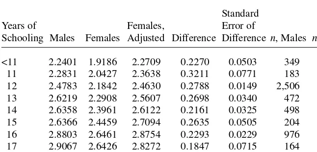
To investigate the relationship between the impact of schooling on earnings and the impact of DTC, a Blinder–Oaxaca decomposition of the earnings gap was performed for each year of schooling, with those respondents with fewer than 11 years, or more than 17, being grouped into single categories. Table 3 shows the mean earnings of males and females by years of schooling, female earnings adjusted for differences in coefficients,11and the unexplained part of the decomposition attributed to DTC.
The index of DTC thus computed for each year of schooling on the whole varies inversely with years of schooling as hypothesized. The estimates for some of the less numerous categories are imprecise but the negative association is confirmed by a descriptive regression of the index on years of schooling that yields a schooling coef-ficient of −0.0136, with tstatistic −54.6.
This negative association is consistent with the hypothesis that a minor but impor-tant side-benefit of schooling for females is that it reduces the gap in male and female earnings attributable to DTC. If this is the case, it would appear inevitable that esti-mates of the returns to schooling will be higher for females than for males in a con-ventional regression specification. The size of the coefficient in the descriptive
regression suggests that about a half of the extra returns to schooling enjoyed by females could be attributed to this effect.
To make the same point in a different way, Column 4 of Table 2 shows the results of controlling for DTC by including the index in the regression specification. Column 5 additionally allows for selectivity. A comparison of Columns 1 and 4, or Columns 3 and 5, suggests that failure to allow for variation in DTC has no effect on the male schooling coefficient but biases upward the female coefficient by approximately one percentage point and accounts for half of the differential in the schooling coefficients. Heckman, Lochner, and Todd (2003) suggest that a wage equation should allow for an interaction between the effects of schooling and experience on earnings. When such a term was added to the specification, together with a further interaction with the female dummy, it was found that it did have a significant coefficient (0.0021, standard error 0.0004), while the female interaction did not (−0.0008, standard error 0.0006). The introduction of these variables caused the estimates of the returns to schooling of those with no experience to be relatively low (0.0236 for males, 0.0526 for females) but it did not otherwise impact on the substance of the findings. For males and females with mean years of work experience, the differential in the schooling coefficients was 0.0190 in the specification without the index of DTC, and 0.0104 in the specification including it. These figures are close to those reported in Columns 1 and 4 of Table 2.
C. Other Possible Causes of the Differential
1. Educational Attainment
Section III suggested several other possible causes of the differential. One was a male-female differential in the quality of educational attainment. If male-females tend to be more motivated students than males and extract more from their time in school, measuring schooling in terms of years of enrollment may mask systematic differentials in the
Dougherty 977
Table 3
Logarithm of hourly earnings by years of schooling
Standard Years of Females, Error of
Schooling Males Females Adjusted Difference Difference n, Males n, Females
quality of schooling attainment, and if the quality of attainment is correlated with years of enrollment, its omission from the regression specification could cause differ-ential biases in the male and female schooling coefficients.
Any measure of academic attainment is inherently arbitrary but for the present pur-poses the type of courses taken in high school, and the grades earned on those courses, were taken as a proxy. It is possible that performance in college may have differed from performance in high school for the 50 percent who enrolled in college, but col-lege transcript data are not available in the NLSY. High school transcripts were collected for most of the civilian NLSY respondents directly from their schools in a supplementary survey undertaken in three rounds over the period 1980–83. The infor-mation collected includes the names of the courses, letter grades, and numbers of credits. The transcripts show that, apart from vocational courses, where females earned more credits than males, the distributions of credits were fairly similar for the sexes. Females did earn uniformly higher average grades, and hence grade points, for all the main subject areas and the differences were significant except in the case of mathematics. However, when the grade point variables, with interactive terms to allow for differences in their impact for males and females, were added to the regression specification, there was no evidence that academic attainment in any discipline impacts on earnings, apart from a positive effect significant at the 5 percent level for science in the case of males. As a consequence, the introduction of grade points had no systematic effect on the coefficients of the other variables.
It is, of course, possible that an effect might have been found if college transcript data had been available. These negative findings are reported because, as Altonji (1995) notes, the number of studies that have attempted to relate high school tran-script data to labor market outcomes is relatively small. Apart from some early stud-ies investigating the impact of vocational education, the NLSY transcript data, in particular, have been little exploited. The present findings appear to be in line with those of Altonji (1995) and Brown and Corcoran (1997).
2. Job Characteristics and Occupational Choice
Another possible reason for a differential in the male-female schooling coefficients is that there might be a composition effect, females being underrepresented in jobs where schooling is a relatively unimportant factor in the determination of earnings. For example, they may be underrepresented among union workers, where schooling is subordinated to seniority as a determinant of earnings, or in self-employment where entrepreneurial skills are relatively highly valued. Alternatively, there may be an occupational effect. There is a consensus in the literature that most of the male-female earnings gap is attributable to the tendency for women to be segregated in occupations with relatively low pay (Treiman and Hartmann 1981; Cain 1986; Gunderson 1989; Chauvin and Ash 1994; Altonji and Blank 1999). In the case of the differential in the male-female schooling coefficients, it was hypothesized that there might also be an occupational effect in that the value of schooling may vary among occupations. The fact that “female” occupations pay relatively poorly does not exclude the possibility that education is valued relatively highly within them.
organization, and self-employment) and union dummy variables were introduced and interacted with the years of schooling variable. To allow for male-female differences, the job characteristic dummy variables, and their interactives with schooling were fur-ther interacted with the female dummy variable.
The results from this specification provided little support for the composition hypothesis. While the estimates of the returns to schooling for males were indeed rel-atively low for the self-employed and for union workers, they also were relrel-atively low for government employees, where males are substantially underrepresented. The overall impact of the introduction of the job characteristic variables on the differen-tial in the male-female schooling coefficients was insignificant.
In a second step, the procedure used for the general job characteristics was extended to include occupations. The introduction of the occupational variables did lead to a marginal reduction (0.0020) in the estimate of the differential in the male-female schooling coefficients. Females were overrepresented among professional workers, where the returns to schooling were high, and underrepresented among most categories of manual worker, where the returns to schooling were low. There was no significant male-female differential in the returns to schooling within occupations, controlling for the general job characteristics.
3. Endogeneity of Schooling and Work Experience
Male-female differentials in the endogeneity of schooling or work experience could in principle account for part of the differential in the estimates of their schooling coef-ficients. Following Korenman and Neumark (1992), tenure and work experience were instrumented using a set of family characteristics: a dummy variable for living with both parents at age 14, a dummy variable for the adult female in the household work-ing for pay when aged 14, mother’s years of schoolwork-ing, father’s years of schoolwork-ing, number of siblings, and desired level of schooling when aged 14. The latter was a sub-stitute for parents’ desired level of schooling for the respondent, not available in the NLSY data set. Dummy variables were included for cases with missing data, the variable in question being set to zero.
The IV results were as pathological as is commonly the case in wage equations. The male schooling coefficient fell to 0.0290 (standard error 0.0126) and the female coefficient rose to 0.0994 (standard error 0.0194), the differential of 0.0703 being sig-nificant at the 1 percent level. Similar but less extreme results were obtained when male tenure and work experience were treated as exogenous. If any weight can be attached to these results, they suggest that endogeneity of tenure and work experience may actually cause estimates of the male-female schooling differential to be biased downward. Given the unsatisfactory nature of the IV results for tenure and work expe-rience, no attempt was made to instrument for schooling.
V. Conclusions
The survey in Section II found that estimates of the returns to schooling in the United States tend to be higher for females than for males, despite the fact that females tend to earn less, both absolutely and controlling for personal
characteristics. Certainly this is so in the case of the NLSY cohort, where the esti-mate of the male-female differential in the schooling coefficients was 0.0196 and highly significant. In a specification that allows for sample selection, the figure is 0.0173.
It was hypothesized that there may be a link between the extra returns to schooling for females and the unexplained part of the gap between male and female log earn-ings. It was found that the log earnings gap is negatively associated with schooling, at least for the NLSY data set. The negative association is imperfect, but a simple descriptive regression of the gap on years of schooling yields a highly significant negative coefficient.
This negative association is consistent with the hypothesis that a minor but impor-tant side-benefit of schooling for females is that it reduces the gap in male and female earnings attributable to factors such as discrimination, tastes, and circumstances. If this is the case, it would appear inevitable that estimates of the returns to schooling will be higher for females than for males in a conventional regression specification. The size of the coefficient in the descriptive regression suggests that about a half of the extra returns to schooling enjoyed by females could be attributed to this effect.
Dougherty
981
Appendix 1
U.S. Studies with Male and Female Schooling Coefficients
Study Dataa DVb Controlsc Findingsd
Altonji (1993) NLS72 1977–1986 H we, we2, family back- Higher female coefficients for both partial college n= 38,595 (no M/F ground, ethnicity, dummy variables, all 8 college degrees, and 5 of breakdown) ability, region the 6 advanced degrees.
Angle and NLS Young Men and H age, family back- M 0.040, F 0.076. Female BA and MA dummy Wissman (1981) Young Women. M 2,831, ground, ethnicity variable coefficients higher but PhD coefficient
F 1,677 lower. Sample restricted to respondents who had
at least some college.
Barron, Black, EOPP 1982 H pwe, training, part- Starting wages: dummy variable coefficients lower and Lowenstein M 683 F 578 time, employer size for females for three categories. Experienced
(1993) wages: lower for two categories.
Blau and Kahn PSID 1980 and 1989 H we, we2, ethnicity 1980: M 0.066, F 0.084, female college and (1997) 1980: M 1,784, F 1,081. advanced degree dummy coefficients also higher.
1989: M 1,591, F 1,149 1989: M 0.090, F 0.083, female college and advanced degree coefficients much higher.
Brown and SIPP for 1984 and NLS72 H Both: we, tenure, SIPP: females have higher coefficients for college Corcoran (1997) 1986. SIPP: subsamples training ethnicity, and postgraduate years of schooling but a lower
from M 8,695, F 7,171 married, SIPP: also coefficient for high school years of schooling NLS72: subsamples from we2, tenure2, child, NLS72: partial college years-of-schooling M 2,635, F 2,359 hsc, region .coefficient higher for females.
NLS72: also ability
The Journal of Human Resources
Appendix 1 (Continued)
Study Dataa DVb Controlsc Findingsd
Card (1999) CPS March 1994–1996. H pwe, pwe2, pwe3, M 0.100, F 0.109 M 102,639, F 95,309 ethnicity
Carlson and 1980 Census, M & F A age, annual hours, Females coefficients for S=12 and S=16 higher for Swartz (1988) 12 ethnic categories married, location of whites, blacks, and 7 other ethnic categories.
residence Male coefficients higher for 3 ethnic categories
Chandler, Kamo, 1987 and 1988 National H we, ethnicity, South, M 0.084, F 0.101, difference reported as significant, and Werbel Surveys of Families and urban, marital delay, size of test not specified.
(1994) Households. years married,
house-M 1,997, F 1,670 work time
Corcoran and PSID 1977. H we, we2, tenure, labor Whites: M 0.059, F 0.077. Duncan (1979) Whites M 2,250, F 1,326. market attachment, Blacks: M 0.061, F 0.076
Blacks M 895, F 741 region
Daymont and NLS72 1979 H we, weeks, married, Relative to college graduates, females have higher Andrisani (1984) M 1,482, F 1,353 job preferences coefficients for master’s and PhD.
Duncan (1996) NLSY 1979–1988 H we, we2, married, Whites: M 0.032, F 0.067 M 34,333, F 30,578 region, urban, hours Blacks: M0.033, F 0.057
per week
Fishback and 1980 Census 1/1000 H pwe, ethnicity, part- M 0.042, F 0.071 Terza (1989) M 12,230, F 9,239 time, region, urban,
Dougherty
983
Gregory, Anstie, CPS March 1982 H pwe, pwe2, married, Relative to high school graduate, females have Daly, and Ho n=13,949; M, F urban higher coefficients for partial college, college
(1989) not given graduates, and postgraduate degree; males have
higher increment from dropouts to high school graduate
Grogger and NLS72 1977–1986 and H we, ethnicity, family Relative to high school graduate, females have Eide (1995) HS&B 1986 (pooled). background, higher coefficients for partial college, college
M 19,597, F 16,223 ability, hsc graduates, and postgraduate degree, the differentials falling with experience
Gronau (1988) PSID 1976 H we, we2, tenure, M 0.060, F 0.069 M 2,398, F 1,936 tenure2, training,
home time, ethnicity, married, region, govt, union
Gwartney and 1960 Census, M and A age, annual hours, Females coefficients for S=12 and S=16 higher for Long (1978) F 9 ethnic categories married, location of whites, blacks, and 5 other ethnic categories
residence Male coefficients higher for 2 ethnic categories
Hersch (1991) Sample from 18 firms in H we, we2, tenure, M 0.041, F 0.056 Eugene, Oregon tenure2, ethnicity,
M 414, F 217 married, child
Hill (1979) PSID 1976 H we, tenure, labor Whites: M 0.062, F 0.074 Whites: M 2,250, force attachment, Blacks: M 0.065, F 0.081
F 1,326 training, annual,
Blacks: M 895, F 741 hours, disability
The Journal of Human Resources
Appendix 1 (Continued)
Study Dataa DVb Controlsc Findingsd
Kane and NLS72 1986 and H Both: we, ethnicity, NLS72: 2-year college M 0.042, F 0.064; 4-year Rouse (1995) NLSY 1990. family background, college M 0.046, F 0.062. NLSY: lower dummy
NLS72: M 3,249, F 3,514. ability, region variable coefficients for females for all educational NLSY: M 2,271, F 2,277 NLS72: also we2 categories except other degree.
NLSY: also age
Loury (1997) NLS72 1979, HS&B 1986 W Both: tenure, weeks, Higher coefficients for females for partial and NLS72: M 1,384, F 1,184. married, union complete college, both data sets.
HS&B: M 732, F 915 worker, hsc
Madden (1978) NLS Young Men and H we, tenure, ethnicity, Whites: M 0.046, F 0.093 Young Women. family background, Blacks M 0.050, F 0.075 Whites M 1,074, F 1,473; region, ability,
Blacks M 453, F 583 married, weeks
Mincer and NLS Mature Women H Married M: we, we2 Married M 0.071, married F 0.063, single F 0.077 Polachek (1974) and SEO, both for 1966 Married F: estimated
(nnot stated). we, tenure, home time. Single F: we, we2, tenure
Murnane, NLS72, 1978 and H we, ethnicity, family NLS72: M 0.013, F 0.037 Willett, and HS&B, 1986. background, part-time HS&B: M 0.021, F 0.037 Levy (1995) NLS72 M 4,114, F 3,925.
Dougherty
985
Neumark (1988) NLS Young Men and H we, age, ethnicity, M 0.062, F 0.072 Young Women, 1980 married, region,
M 1,819, F 1,505 urban, union worker
Oaxaca (1973) SEO 1967. H pwe, pwe2, married, Uses a quadratic for years-of-schooling Whites: M 8,123, F 4,962. urban, region, Whites: females have lower implicit coefficients Blacks: M 3,897, F 3,502 part-time Blacks: females have higher implicit coefficients
Rosenzweig 1970 Census, 1 in 10,000 H pwe, pwe2 M 0.078, F 0.116 (1976). sample. M 3,251, F 375
Rumberger and NLSY 1980 H pwe, ethnicity, M 0.047, F 0.055. Sample restricted to those who Daymont (1984) M 713, F 648 married, ability, child did not complete a year of college
Wellington PSID 1976, 1985. H we, we2, tenure, 1976: M 0.049, F 0.074 (1993) 1976: M 1,535, F 1,002. training, home time, 1985: M 0.062, F 0.079
1985: M 1,901, F 1,544 labor force, attachment, region, urban
Notes:
a.Data:M male, F female, with numbers of observations. For data set abbreviations, see section 3. b.DV (dependent variable):H hourly wage, W weekly earnings, A annual earnings, in each case logarithmic.
c.Controls:we: work experience; pwe: potential work experience; child: number of children or presence of a child in the household; hsc: high school courses or grades; urban: resides in urban area, or SMSA, or city size; weeks: weeks worked in the year; govt: works in public sector.
Appendix 2
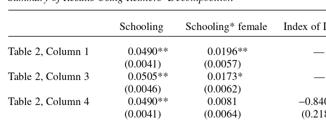
Summary of Results Using Reimers’ Decomposition
Schooling Schooling* female Index of DTC
Table 2, Column 1 0.0490** 0.0196** — (0.0041) (0.0057)
Table 2, Column 3 0.0505** 0.0173* — (0.0046) (0.0062)
Table 2, Column 4 0.0490** 0.0081 −0.8405**
(0.0041) (0.0064) (0.2182) Table 2, Column 5 0.0505** 0.0047 −0.9377**
(0.0046) (0.0070) (0.3208)
The table shows the schooling coefficients corresponding to those reported in Table 2 with an index of DTC using Reimers’ decomposition of the male-female earnings gap. The coefficient of the index of DTC is larger with the Reimers decomposition than with the Oaxaca decomposition. This is attributable to the smaller vari-ance in the index when computed in this way. The introduction of the index causes a slightly larger reduc-tion in the male-female differential in the schooling coefficients than in the case of the Blinder-Oaxaca version.
References
Altonji, Joseph G. 1993. “The Demand for and Return to Education when Education Outcomes are Uncertain.” Journal of Labor Economics11(1, part 1):48–83
———. 1995. “The Effects of High School Curriculum on Education and Labor Market Outcomes.” Journal of Human Resources30(3):409–38.
Altonji, Joseph G., and Rebecca M. Blank. 1999. “Race and Gender in the Labor Market.” In
Handbook of Labor Economics, Vol 3ed. Orley Ashenfelter and David Card, 3143–3259. Amsterdam: Elsevier .
Angle, John, and David A. Wissman. 1981. “Gender, College Major, and Earnings.” Sociology of Education54:25–33
Baltagi, Badi H. 2001. Econometric Analysis of Panel Data(second edition), Chichester, U.K.: John Wiley.
Barron, John M., Dan A. Black, and Mark A. Loewenstein. 1993. “Gender Differences in Training, Capital, and Wages.” Journal of Human Resources28(2):343–64.
Blau, Francine D., and Andrea H. Beller. 1988. “Trends in Earnings Differentials by Gender.”
Industrial and Labor Relations Review41(4):513–29.
Blau, Francine D., and Lawrence M. Kahn. 1992. “Race and Gender Pay Differentials.” In
Research Frontiers in Industrial Relations and Human Resourcesed. David Lewin, Olivia S. Mitchell, and Peter D. Sherer, 381–415. Madison, Wis.: Industrial Relations Research Association
———. 1997. “Swimming Upstream: Trends in the Gender Wage Differential in the 1980s.”
Journal of Labor Economics15(1, part 1):1–42
———. 2000. “Gender Differences in Pay.” Journal of Economic Perspectives, 14(4):75–99. Blinder, Alan S. 1973. “Wage Discrimination: Reduced Form and Structural Estimates.”
Journal of Human Resources8(4):436–55.
Cain, Glen G. 1986. “The Economic Analysis of Labor Market Discrimination: a Survey.” In Handbook of Labor Economics, Vol 1, ed. Orley Ashenfelter and Richard Layard, 693–785. Amsterdam: Elsevier Science Publishers.
Card, David. 1999. “The Causal Effect of Education on Earnings.” In Handbook of Labor
Economics, Vol. 3, ed. Orley Ashenfelter and David Card, 1801–63. New York: Elsevier. Carlson, Leonard A., and Caroline Swartz. 1988. “The Earnings of Women and Ethnic
Minorities, 1959–1979.” Industrial and Labor Relations Review41(4):530–46.
Chandler, Timothy D., Yoshinori Kamo, and James D. Werbel. 1994. “Do Delays in Marriage
and Childbirth Affect Earnings?” Social Science Quarterly75(4):838–53.
Chauvin, Keith W., and Ronald A. Ash. 1994. “Gender Earnings Differentials in Total Pay,
Base Pay, and Contingent Pay.” Industrial and Labor Relations Review47(4):634–49.
Cohen, Malcolm S. 1971. “Sex Differences in Compensation.” Journal of Human Resources
6(4):434–47.
Corcoran, Mary, and Greg J. Duncan. 1979. “Work History, Labor Force Attachment, and
Earnings Differences between the Races and Sexes.” Journal of Human Resources
14(1):3–20.
Cotton, Jeremiah. 1988. “On the Decomposition of Wage Differentials.” Review of Economics
and Statistics70(2):236–43.
Duncan, Kevin C. 1996. “Gender Differences in the Effect of Education on the Slope of the
Experience-Earnings Profiles.” American Journal of Economics and Sociology
55(4):457–71.
Featherman, David L., and Robert M. Hauser. 1976. “Sexual Inequalities and Socioeconomic
Achievement in the U.S., 1962–1973.” American Sociological Review41(3):462–83.
Fishback, Price C., and Joseph V. Terza. 1989. “Are Estimates of Sex Discrimination by
Employers Robust? The Use of Never-Marrieds.” Economic Inquiry27(2):271–85.
Gregory, Robert G., Roslyn Anstie, Anne Daly, and Vivian Ho. 1989. “Women’s Pay in Great Britain, Australia, and the United States: the Role of Laws, Regulations, and Human
Capital.” In Pay Equity: Empirical Inquiries, ed. Robert T. Michael, Heidi I. Hartmann, and
Brigid O’Farrell, 222–42. Washington D.C.: National Academy Press
Grogger, Jeff, and Eric Eide. 1995. “Changes in College Skills and the Rise in the College
Wage Premium.” Journal of Human Resources30(2):280–310.
Gronau, Reuben. 1988. “Sex-Related Wage Differentials and Women’s Interrupted Labor
Careers—the Chicken or the Egg.” Journal of Labor Economics6(3):277–301.
Grubb, W. Norton. 1993. “The Varied Economic Returns to Postsecondary Education.” Journal of Human Resources28(2):365–82.
Gunderson, Morley. 1989. “Male-Female Wage Differentials and Policy Responses.” Journal
of Economic Literature27(1):46–72.
Gwartney, James D., and James E. Long. 1978. “The Relative Earnings of Blacks and Other
Minorities.” Industrial and Labor Relations Review31 (3):336–46.
Heckman, James J. 1980. “Sample Selection Bias as a Specification Error with an Application
to the Estimation of Labor Supply Functions.” In Female Labor Supply: Theory and
Estimation, ed. James P. Smith, 206–48. Princeton, N.J: Princeton University Press. Heckman, James J., Lance J. Lochner, and Petra E. Todd. 2003. “Fifty Years of Mincer
Earnings Regressions.” Working Paper 9732, National Bureau of Economic Research Heckman, James J., and Solomon Polachek. 1974. “Empirical Evidence on the Functional
Form of the Earnings-Schooling Relationship.” Journal of the American Statistical
Association69(346):350–54.
Hersch, Joni. 1991. “Male-Female Differences in Hourly Wages: the Role of Human Capital,
Working Conditions, and Housework.” Industrial and Labor Relations Review44(4):746–59.
Hill, Martha S. 1979. “The Wage Effects of Marital Status and Children.” Journal of Human
Resources14 (4):579–94.
Hirschberg, J.G., and D.J. Slottje. (2002) “Bounding Estimates of Wage Discrimination.” Working paper No. 879, Department of Economics, University of Melbourne.
Hsiao, Cheng. 2002. Analysis of Panel Data(second edition). Cambridge: Cambridge
University Press.
Jones, F. L. 1983. “On Decomposing the Wage Gap: a Critical Comment on Blinder’s
Method.” Journal of Human Resources18(1):126–30.
Kane, Thomas J., and Cecilia E. Rouse. 1995. “Labor-Market Returns to Two- and Four-Year
College.” American Economic Review85(3):600–14.
Kenny, Lawrence W., Lung-Fei Lee, G. S. Maddala, and R. P. Trost. 1979. “Returns to College Education: an Investigation of Self-Selection Bias Based on the Project Talent
Data.” International Economic Review20(3):775–89.
Korenman, Sanders, and David Neumark. 1992. “Marriage, Motherhood, and Wages.” Industrial and Labor Relations Review50(4):580–93.
Madden, Janice F. 1978. “Economic Rationale for Sex Differences in Education”, Southern
Economic Journal44(4):778–97.
———. 1985. “The Persistence of Pay Differentials: the Economics of Sex Discrimination.” In Women and Work: an Annual Review, ed. Laurie Larwood, Ann H. Stromberg, and Barbara A. Gutek, 76–114. Beverley Hills, Calif.: Sage.
Mincer, Jacob, and Solomon Polachek. 1974. “Family Investments in Human Capital:
Earnings of Women.” Journal of Political Economy82(2, part 2):S76–S108.
Murnane, Richard J., John B. Willett, and Frank Levy. 1995. “The Growing Importance of
Cognitive Skills in Wage Determination.” Review of Economics and Statistics
77(2):251–66.
Neumark, David. 1988. “Employers’ Discriminatory Behavior and the Estimation of Wage
Discrimination.” Journal of Human Resources23(3):279–95.
Oaxaca, Ronald L. 1973. “Male-Female Wage Differentials in Urban Labor Markets.” International Economic Review14(3):693–709.
Oaxaca, Ronald L., and Michael R. Ransom. 1994. “On Discrimination and the Decomposition
of Wage Differentials.” Journal of Econometrics61(1):5–21.
———. 1999. “Identification in Detailed Wage Decompositions.” Review of Economics and
Statistics81(1):154–57.
O’Neill, June, and Solomon Polachek. 1993. “Why the Gender Gap in Wages Narrowed in the
1980s.” Journal of Labor Economics11(1):205–28.
Reimers, Cordelia W. 1983. “Labor Market Discrimination Against Hispanic and Black Men” Review of Economics and Statistics65(4):570–79.
Roos, Patricia A. 1981. “Sex Stratification in the Workplace: Male-Female Differences in
Economic Returns to Occupation.” Social Science Research10(3):195–223.
Rosenzweig, Mark R. 1976. “Nonlinear Earnings Functions, Age, and Experience: A
Nondogmatic Reply and Some Additional Evidence.” Journal of Human Resources
11(1):23–27.
Rumberger, Russell W. and Thomas N. Daymont. 1984. “The Economic Value of Academic
and Vocational Training Acquired in High School.” In Youth and the Labor Market, ed.
Michael E. Borus, 157–91. Kalamazoo: W. R. Upjohn Institute for Employment Research. Suter, Larry E., and Herman P. Miller. 1973. “Income Differences between Men and Career
Women.” American Journal of Sociology78(4):962–74.
Treiman, Donald J., and Heidi I. Hartmann, eds. 1981. Women, Work, and Wages: Equal Pay
for Jobs of Equal Value. Washington, D.C.: National Academy Press
Trostel, Philip, Ian Walker, and Paul Woolley. 2002. “Estimates of the Economic Return to
Schooling for 28 Countries.” Labour Economics9(1):1–16.
Wellington, Alison J. 1993. “Changes in the Male/Female Wage Gap, 1976–1985.” Journal of